
Manually searching a huge spreadsheet for specific content might be tedious. In Google Sheets, there is no exact IF CONTAINS formula. However, you may automate the procedure by using a creative combination of a few formulae.
This article will walk you through using various formulae to search a cell to determine if it has a particular value or not. Continue reading to learn how to grasp IF contains Google Sheets functions and formulas using the Sheets Tips provided on this page.
IF Cell Contains using REGEXMATCH
The REGEXMATCH function is one of the finest ways to search your data to determine if a cell has a specific value.
This function will search a cell for the text that fits your regular expression and return TRUE if it does, or FALSE if it does not.
Also Read: Python Program to Count Non Palindrome words in a Sentence
This function’s syntax is as follows:
REGEXMATCH(text, regular_expressions)
The text is the text or reference to the cell you are looking for.
The text or values you are looking for are represented by regular expressions. As the second parameter, you put the text you wish to search for inside quote marks. You may also use the sign “|” to search for multiple items.
Here’s how to use this method to check if a cell contains a certain value:
- Step 1: To begin your formula, choose the cell where you wish the formula to be evaluated and type =REGEXMATCH.
- Step 2: The first parameter is the cell you wish to search. Select the cell to be searched and enter a comma (,)
- Step 3: The second option is the text you want to find. Put your text within quote marks and finish with the parentheses “)”
- Step 4: Press ENTER and copy your formula to any further cells where you wish to repeat it.
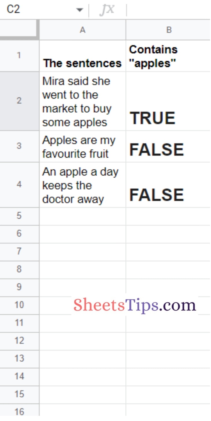
The formula returns either TRUE or FALSE. In this example, any cell containing the word “apples” returns TRUE because that is what my REGEXMATCH algorithm is configured to look for.
The REGEXMATCH function is really handy, but there are a few things to keep in mind regarding how it operates.
The first thing to remember is that it is case-sensitive. If your term is capitalized differently from what you are looking for, it will always return FALSE.
There are two techniques to search for every iteration of the text, regardless of whether it is capitalized or not.
- Using the or symbol (|) – The or symbol (|) may be used in your formula to search for several items. To utilize it in the previous example, alter your formula to =REGEXMATCH(A2,”apples|Apples”). If your cell contains the words apples OR Apples, this function will return true.
- Using the LOWER function – Another brilliant method is to use the LOWER function in your calculation to change your text to lowercase before searching it. Change your formula to =REGEXMATCH(lower(A2),”apples”). This is a superior way because you won’t have to bother about capitalization.
IF Cell Contains using IF & SEARCH
Another creative method for determining if a cell has a specific number or text is to combine the IF and SEARCH Functions.
You would pair them using the following syntax:
=IF(SEARCH(“your text”, A2) > 0, 1, 0)
This formula will determine if the cell you are looking for (A2) has your “text.” If it matches, the formula will evaluate to 1, else an error message will display saying #VALUE!
The benefit of this formula is that it can also be used to search for numbers without the need to style your cell as text as in the previous example.
Here’s how you’d put it to use:
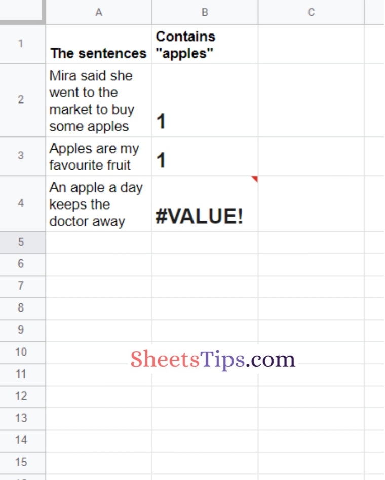
As seen in this case I’m looking for my text “apples” in cell A2. If the cell has it, the formula evaluates to 1, else it displays #VALUE!
This approach is superior to the prior method. This formula is not case-sensitive and may be used to search for numbers.
IF Cell Contains using COUNTIF
Another possibility is using the COUNTIF function.
This formula will be written in the following syntax:
=COUNTIF(A2,“*your text*”)
That formula will search your cell and return 1 if it finds your text; else, it will return 0.
You must include an asterisk (*) around the text you are looking for since this represents a wildcard in your calculation. This indicates it will seek for your text anywhere in the cell rather than simply an exact match on your full cell.
Here’s how you’d use it in a formula to find a cell:
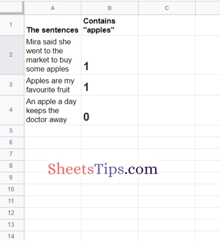
In this case, I’m looking to check if the cell contains the word “apples.” If it does, the formula returns a 1, else it returns a 0.
This approach does not search numbers and is not case-sensitive.
If you wish to search for a number, you must first convert the cell to text for the formula to operate properly.
These methods for determining if a cell contains a certain string of text are quite useful. Each approach has advantages and disadvantages, but they may all be employed to achieve the same outcome.
We urge that you practice and attempt to learn how to apply each strategy and why it works.
We hope you found this information useful!
Must Read: