
Google Sheets is an excellent online software solution for creating and organizing spreadsheets. The SORTN Google Sheets function, which allows you to sort an “n” number of objects, is one such function. This post will go through what the function is, how it works, and how to use it using the Google Sheets tips provided on this page. Continue reading to learn how to use these SORTN functions in Google Sheets.
- What Is SORTN in Google Sheets?
- What Is the SORTN Google Sheets Function?
- How To Use SORTN Google Sheets Function?
- Error Handling with the SORTN Function
What Is SORTN in Google Sheets?
The SORTN formula in Google Sheets allows you to sort a range of data. It retrieves the first “n” items from that range. As a result, it’s literally “sort n.” If no number is given, the formula will return the least value (1).
Using this technique drastically decreases the number of steps required to identify a value in a table and sort your data.
In nature, SORTN is quite similar to the FILTER function. SORTN, on the other hand, returns the largest “n” amount, whereas FILTER returns the matched rows.
Also Read: Python Program to Print the Equilateral Triangle Pattern of Star
What Is the SORTN Google Sheets Function?
SORTN’s formula is extremely lengthy since it has many more references than many other functions. Let’s start with the syntax to assist you to comprehend the formula. The Google Sheets SORTN structure is as follows:
=SORTN(range, [n], [display-ties-mode], [sort-column1, is-ascending1], …)
The following parameters are utilized in this formula:
- range – The data you wish to sort is in this range.
- n- The item number in the dataset you want to return is represented by the optional parameter n. It should always be larger than zero and is 1 by default.
- When there is a tie in the data being sorted, the display-ties-mode parameter specifies which items will be displayed. This might range from 0 to 3. What the choices do is as follows:
- 0 – At most, only display the first “n” rows in the range.
- 1 – This displays the first “n” rows. There will also be more rows that are comparable to the nth number of rows.
- 2 – After eliminating duplicate rows, this displays the first “n” rows.
- 3 – This displays the first “n” rows along with duplicates of those rows.
- Sort-column1- This input, sort-column1, is likewise optional. These are the column’s cells in the range or outside range that contain the values needed to order it.
- is-ascending1 –Choose whether to sort your data in an ascending or descending manner using the optional argument is-ascending1. When this option is set to TRUE, data are sorted in ascending order; when set to FALSE, data are sorted in descending order.
- sort-column2 – Similar to sort column1, sort-column2 is an optional parameter that performs the same function. There is no limit to how many sort columns you may add.
- is-ascending2 – You may define whether the sort-column2 is ascending or descending with the optional parameter is-ascending2.
How To Use SORTN Google Sheets Function?
It is recommended to use an example to illustrate the SORTN function in Google Sheets so that you can grasp it better. For this presentation, we will use the following sample set of data:
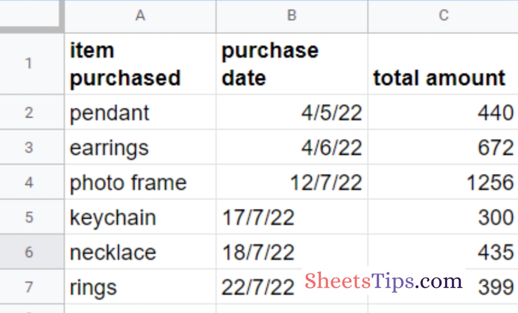
We want to sort the items with the most expensive item sold, and we only wish to show the top 3 items.
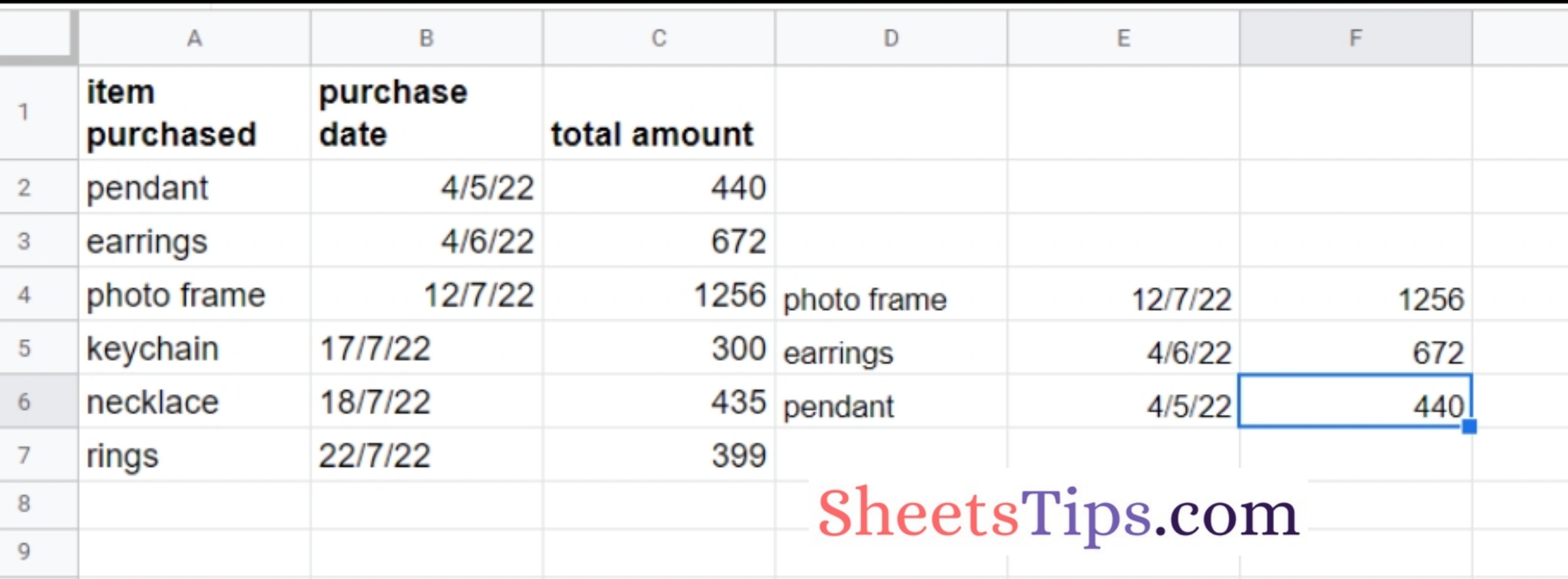
Here is what the formula will look like in this particular case:
=SORTN(A2:C8,3,0,C2:C8,FALSE)
After using the formula, the outcome should be like this:
Let’s examine what each argument in this example of the formula does:
- The range we want to include in the SORTN formula is A2:C8.
- 3 – This number represents the number of units that we want to display after sorting. Only the top three things should be displayed. Consequently, the answer is 3.
- 0 – The handling of ties is specified by this parameter. Since we’ve set it to 0, a maximum of the first “n” rows will be shown.
The column that was utilized to order the data is designated by the range C2:C8. By using the information beneath the Total Amount column, we may order our data according to the highest price.
Error Handling with the SORTN Function
These are some of the mistakes you could make while using the SORTN function. And solutions for how to solve them.
- #REF! – The message that appears on the screen reads, “Array result was not enlarged because it might overwrite data in…” When the cell doesn’t have enough room to display the data, an error might happen. The output cannot be shown because of either the cells below or the cells to the right. To correct this problem, think about removing the data from the blocking cells or relocating the data to another cell.
Additionally, you could have entered your data into the calculation improperly, resulting in a circular dependency problem.
- #VALUE! – When the input is not a continuous range of cells, this error is shown. The cell ranges A1:A4 and A6:A9 might contain some data. Consider modifying such that all the data occurs in a single cell range.
Many people work in the banking sector, where they must arrange a lot of data. However, they are not the only users who would gain from this. Many users may find the SORTN Google Sheets tool to be quite beneficial in a variety of circumstances.
Making use of this feature might help you handle data effectively. Data may be sorted by the frequency of appearances with ease using the Google Sheet SORTN function.
Must Read: