Google Sheets Tips: Even if you use spreadsheets regularly, you may not be aware of the width and depth of their capabilities. This is true with Google Sheets in particular! Google has been developing Google Sheets since 2006 as part of its Google Workspace formerly known as G-Suite. Today, Google Sheets is an attractive solution to rapidly analyze and treat data, because it requires quick and easy collaboration worlds.
On this page, we will summarize a list of tips and tricks you must learn today to increase your Google Sheets skills quickly. Scroll down and explore the hacks to use the Google Spreadsheet like a pro!!
Latest Google Sheets Tips
- Keyboard Shortcuts for Google Sheets
- Insert Bullets in Google Sheets
- Add Heatmaps Using Conditional Formatting
- Send Emails when you Comment in Google Sheet
- How to Apply Filters in Google Sheet
- Clean Up Values with CLEAN and TRIM
- Protect Data in Cells
- Validate Data in Cells
- Integrate Google Sheet with Google Forms
- Insert a Chart from Google Sheets into a Google Doc
- Import data from a website or RSS feed To Google Sheet
- Change Capitalization in Cells
- Translate Text in Google Sheet
- Split names and other data
- Check for valid email address
- Spell Check in Google Sheet
- Import data from other sheets
- Visualize data with a sparkling
- Create QR codes
- Check if the Cell is Really Blank
- Extend Google Sheets with add-ons
- Quickly learn formula
- Wrap Text in Google Sheets
Edit & Format a Spreadsheet
- Edit & format a spreadsheet
- Edit and View Text from Right to Left
- Add, Edit, View, Filter and Delete Comments
- Merge Cells in Google Sheets
- Freeze / Lock Rows in Google Sheets
- Lock Cells in Google Sheets (Protect a Range)
- How to Protect Your Google Spreadsheet Data?
- Round Numbers in Google Sheets (ROUNDUP/ROUNDDOWN)
- Format Phone Numbers In Google Sheets
- Convert Text to Numbers In Google Sheets
- Multiply Numbers in Google Sheets (Multiply Rows, Columns or Cells in Google Sheets)
- Divide in Google Sheets (Divide Numbers, Columns, Rows, Multiple Cells)
- SUM a Column in Google Sheets (Add Numbers, Row, Columns, Cells)
- How to Insert an Image in a Cell in Google Sheets
- Add or move columns & cells
- Protect, hide, and edit sheets
- Set a spreadsheet’s location & calculation settings
- Add an image to a spreadsheet
Use functions & formulas
- Google Sheets function list
- How to Use MODE Function in Google Sheets?
- How to Use the ISTEXT Function in Google Sheets
- How to Use REGEXEXTRACT Google Sheets Function
- How to Use REGEXREPLACE Function in Google Sheets
- How to Use SWITCH function in Google Sheets?
- Google Sheets Weekday Function – Explained with Examples
- Using FILTER Function in Google Sheets (explained with Examples)
- How to Use OR Function in Google Sheets (with Examples)
- How to Use IMPORTRANGE Function in Google Sheets (with Examples)
- How to Use IMPORTDATA function in Google Sheets
- Using IFS Function in Google Sheets to Test Multiple Conditions
- Using IFERROR Function in Google Sheets (with Examples)
- How to Use the INDEX function in Google Sheets (Examples)
- Google Sheets Features 2022: Check Five Most Commonly Used Functions in Google Sheets
- How to Show Formulas Instead of Values in Google Sheets
- How to See Basic Calculations Without Formulas in Google Sheets?
- How to SUM a Column in Google Sheets? (Add Numbers, Row, Columns, Cells)
- How To Calculate Weighted Average In Google Sheets (AVERAGE.WEIGHTED)?
- Using IF Function in Google Sheets (with Examples)
- Using Query Function in Google Sheets – Examples
- How to Use COUNTIF Function in Google Sheets
- How to VLOOKUP from Another Sheet in Google Sheets
- The Ultimate Guide to Google Sheets VLOOKUP Function (with Examples)
Work with Data
- Create & use pivot tables
- How to Refresh Pivot Table in Google Sheets
- How to Use Slicer in Pivot Tables in Google Sheets
- How to Add & Use Calculated Fields in Google Sheets Pivot Tables
- How to Group by Month in Pivot Table in Google Sheets
- Auto Suggested Pivot Chart in Google Sheets
- How To Unpivot Table in Google Sheets?
- Reference data from other sheets
- Using arrays in Google Sheets
- How to Import and Open CSV File in Google Sheets
- How to Use IMPORTRANGE Function in Google Sheets
- How to Use IMPORTDATA function in Google Sheets?
- How to Use IMPORTFEED in Google Sheets
- Automatically create a series or list
- Name a range of cells
- Display KPIs with scorecard charts
Sort, filter, or format data
- How to Sort by Color in Google Sheets
- How to Sort Data in Google Sheets
- How to Create Filter Views in Google Sheets?
- How to Use Filter Functions in Google Sheets with Examples
- How To Filter Google Sheets Data Without Changing What Collaborators See?
- How to Create a Dependent Drop Down List in Google Sheets
- How to Create a Drop Down List in Google Sheets
- Conditional Formatting Based on Another Cell Value in Google Sheets
- The Ultimate Guide to Using Conditional Formatting in Google Sheets
- How to Split Text to Columns in Google Sheets
- How to Remove Duplicates in Google Sheets?
- Data Cleaning in Google Sheets
- How to Insert Checkbox in Google Sheets
Create and Edit Charts
- Add & edit a chart or graph
- Add & edit a trendline
- Dynamic Chart Banding in Google Sheets
- Radial Bar Chart in Google Sheets Example
- How to Create a Grid Chart in Google Sheets?
- Funnel Charts In Google Sheets
- How to Make a Line Chart in Google Sheets
- How to Make a Pie Chart in Google Sheets
- How to Create Candlestick Chart in Google Sheets
- How to Make Dot Plot in Google Sheets?
- How To Sync Charts From Google Sheets to Google Docs & Google Slides?
- How to Create a Gantt Chart in Google Sheets?
- How To Switch Chart Axes in Google Sheets?
- How to Make an Organization Chart in Google Sheets?
- How To Create Multi Colored Line Charts in Google Sheets?
- How To Create a Waterfall Chart in Google Sheets?
- How to Make a Histogram in Google Sheets
- How to Make a Bell Curve in Google Sheets
Print or Publish a spreadsheet
Shortcuts & Troubleshooting
- Use Google products side by side
- Automate tasks in Google Sheets
- Troubleshoot Google Docs, Sheets, Slides & Forms error message: “Something went wrong”
- Keyboard shortcuts for Google Sheets
- Turn on notifications in a spreadsheet
- Use Smart Fill in Sheets to automate data entry
- Use Dark theme in Google Docs, Sheets & Slides
- Use Sheets Smart Cleanup to prepare your data for analysis
- Troubleshoot error message in Google Sheets: “Can’t save your changes. Please copy your recent edits then revert your changes.”
Improve Your Sheets Performance
- Learn more about Import functions
- Learn how to improve Sheets performance
- Optimize your data references to improve Sheets performance
Tools
- Use add-ons, Apps Script & AppSheet
- Import, edit & sync Salesforce data with Google Sheets
- Find an unknown value with Goal Seek
- Import and analyze Zendesk data with Google Sheets
- Google Workspace Add-ons
Use BigQuery data in Google Sheets
- Get started with BigQuery data in Google Sheets
- Sort & filter BigQuery data in Google Sheets
- Analyze & refresh BigQuery data in Google Sheets using Connected Sheets
- Write & edit a query
- Fix problems with BigQuery data in Google Sheets
Google Sheets Tips and Tricks
- How to Use the ISTEXT Function in Google Sheets
- How to Make a Dot Plot in Google Sheets
- Edit and View Text from Right to Left
- Use Dark Theme in Google Sheets
- How to Add Labels to Legend in Google Sheets (Step-by-Step)
- How to Hide Columns from Certain Users in Google Sheets
- How to Use Index Match in Google Sheets (Step-by-Step Guide)
- Add, Edit, View, Filter and Delete Comments
- How to Use REGEXEXTRACT Google Sheets Function
- What-If Analysis in Google Sheets Using Goal Seek
- How to Use REGEXREPLACE Function in Google Sheets
- How to Get Running Totals in Google Sheets (Easy Formula)
- Creating Candlestick Chart in Google Sheets (Step-by-step)
- How to Use the INDEX function in Google Sheets (Examples)
- Using Wildcards in Google Sheets (4 Examples)
- How to Combine Formula and Text in Google Sheets
- How to Convert PDF to Google Sheets
- How to Convert Text to Date in Google Sheets
- How to Convert Formula to Value in Google Sheets
- How to Use Slicer in Pivot Tables in Google Sheets
- How to Group Columns in Google Sheets
- How to Convert Time to Decimal in Google Sheets
- Comparison Operators in Google Sheets (A Complete Guide)
- Formula Parse Error in Google Sheets (& How to Fix it)
- How to Add & Use Calculated Fields in Google Sheets Pivot Tables
- How to Group by Month in Pivot Table in Google Sheets
- How to Refresh Pivot Table in Google Sheets
- How to Delete Every Other Row in Google Sheets (Easy Formula Trick)
- How to Make a Bell Curve in Google Sheets?
- How to Import and Open CSV File in Google Sheets?
- How to Convert Time to Military Time Format in Google Sheets?
- How to Use SWITCH function in Google Sheets?
- How to Round Numbers in Google Sheets? (ROUNDUP/ROUNDDOWN)
- How to Print Labels from Google Sheets (For Free)
- How To Calculate Weighted Average In Google Sheets (AVERAGE.WEIGHTED)?
- How to Make a Scatter Plot in Google Sheets (Step-by-Step)
- Turn on Notifications in a Spreadsheet
- How To Format Phone Numbers In Google Sheets?
- How To Recover Deleted Google Sheets Files
- How To Move A Column In Google Sheets
- How to Set Print Area in Google Sheets
- How to Unhide Rows in Google Sheets (4 Easy Methods)
- How to Show Formulas Instead of Values in Google Sheets
- Format Painter in Google Sheets (Copy formatting easily)
- How to Highlight Duplicates In Google Sheets (Easy Steps)
- How to Strikethrough in Google Sheets (3 Easy Ways + Shortcut)
- How to VLOOKUP from Another Sheet in Google Sheets
- How to Convert Text to Numbers In Google Sheets
- How to Compare Two Columns in Google Sheets (for matches & differences)
- How to Make a Histogram in Google Sheets (Step-by-Step)
- How to Make a Line Chart in Google Sheets (Step-by-Step)
- How to Sort by Color in Google Sheets
- How to Make a Pie Chart in Google Sheets (Step-by-Step)
- How to Automatically Send Emails from Google Sheets (Using Appscript)
- How to Insert a Pivot Table in Google Sheets (Step-by-Step)
- Capitalize First Letters in Google Sheets (Easy Formula)
- Remove Last Character from a String in Google Sheets (or Last N Characters)
- Leave Tracker Template in Google Sheets (Updated for 2021)
- Sparkline in Google Sheets – The Only Guide You Need
- Show / Hide Gridlines in Google Sheets (in less than 5 seconds)
- How to Insert Timestamp in Google Sheets
- How to Insert Checkbox in Google Sheets (with Examples)
- 101 Google Sheets Keyboard Shortcuts
- How to Insert Spin Button in Google Sheets (+1 Increment Buttons)
- How to Copy a Sheet from One Google Sheets to Another
- 4 Steps for Quick and Easy Data Analysis with Google Sheets
- How to Create and Use Filter Views in Google Sheets
- How to Create a Table of Contents in Google Sheets
- Google Sheets Weekday Function – Explained with Examples
- How to Get the Last Monday of the Month in Google Sheets
- Calculate Age in Google Sheets (using the Date of Birth)
- How to Create Hyperlinks in Google Sheets (Step-by-Step Guide)
- Using FILTER Function in Google Sheets (explained with Examples)
- How to Search in Google Sheets and Highlight the Matching Data
- How to Use OR Function in Google Sheets (with Examples)
- How to Use IMPORTRANGE Function in Google Sheets (with Examples)
- How to Use IMPORTDATA function in Google Sheets
- Calculate the Number of Days Between Two Dates in Google Sheets
- Using IFS Function in Google Sheets to Test Multiple Conditions
- How to Quickly Freeze / Lock Rows in Google Sheets
- Using IFERROR Function in Google Sheets (with Examples)
- How to Create a Drop Down List in Google Sheets
- Using IMPORTFEED in Google Sheets to Fetch Feed from URL
- Using Query Function in Google Sheets – Examples
- Concatenate in Google Sheets – Combine Cells Using Formula
- How to Zoom In and Zoom Out in Google Sheets
- How to Quickly Transpose Data in Google Sheets
- How to Fill Down in Google Sheets Using Fill Handle
- Calendar Template in Google Sheets (Monthly and Yearly)
- The Ultimate Guide to Google Sheets VLOOKUP Function (with Examples)
- How to Create Named Ranges in Google Sheets (Static & Dynamic)
- How to Quickly Insert Multiple Rows in Google Sheets
- How to Rotate Text in Google Sheets (in less than 5 seconds)
- How to Count Cells If Not Blank in Google Sheets
- Conditional Formatting Based on Another Cell Value in Google Sheets
- Creating a Heat Map in Google Sheets (Step-by-Step Tutorial)
- How to Split Text to Columns in Google Sheets (with Examples)
- How to Convert Excel to Google Sheets (a Step-by-Step Tutorial)
- How to Create a Dependent Drop Down List in Google Sheets
- How to Insert an Image in a Cell in Google Sheets
- How to Use COUNTIF Function in Google Sheets
- How to Quickly Merge Cells in Google Sheets
- The Ultimate Guide to Using Conditional Formatting in Google Sheets
- How to Use Spell Check in Google Sheets to Find Misspelled Words
- Using IF Function in Google Sheets (with Examples)
- How to Lock Cells in Google Sheets (Protect a Range)
- How to Sort Data in Google Sheets
- How to Wrap Text in Google Sheets
- How to Insert Bullets in Google Sheets
- How to Count the Number of Words in Google Sheets
- How to Remove Duplicates in Google Sheets
- How to Color Alternate Rows in Google Sheets
- How to Add ColourFul Stripes in Google Sheets?
- How to Open Google Sheet on a Specific Tab?
- Google Spreadsheet Limitations
- How to Gain Insights to Your Google Sheets Data via Explore
- How to Manage Date in Google Spreadsheet with List View?
- How to Protect Your Google Spreadsheet Data?
- How to Resize Rows and Columns in Google Sheets?
- How to Make Tables in Google Sheets?
- How to Apply a Color Scale Based on Values in Google Sheets?
- How to Convert Currency in Google Sheets?
- How to Insert a Google Sheets Into Google Docs?
- How To Create Star Rating System in Google Sheets?
- How to Sync Data From One Google Sheet to Another Spreadsheet?
- How to View Activity Dashboard in Google Sheets
- Named Versions in Google Sheets
- How to Add Text Rotation and Perform Accounting in Google Sheets?
- Google Spreadsheet Locale Settings
- How to Remove Zero Value from Google Spreadsheet?
- Auto Suggested Pivot Tables in Google Sheets
- How to Add or Remove Rows and Columns in Google Spreadsheet? (With Keyboard Shortcuts)
- How to Open Links in Google Sheets with Single Click – Google Sheets Clickable Cell
- How to Multiply Numbers in Google Sheets? – Multiply Rows, Columns or Cells in Google Sheets
- How to Publish Google Sheets as Web Page: Share Google Sheets to Public
- How to Divide in Google Sheets? (Divide Numbers, Columns, Rows, Multiple Cells)
- How to SUM a Column in Google Sheets? (Add Numbers, Row, Columns, Cells)
- How to Hide Tabs or Spreadsheets in Google Sheets? (Hide or Unhide Sheets)
- How To Open Google Spreadsheet in New Window? (View Two Tabs at Once)
- How to Convert Rows to Columns or Backwards in Google Sheets?
- How To Assign Tasks in Google Sheets? (Enable Tasks Using Comments)
- How to See Basic Calculations Without Formulas in Google Sheets?
- How to Use Paste Special Options in Google Spreadsheet? Google Sheets Paste Special Explained
- How to Present Google Sheets in Google Meet -2 Easy Methods to Present Google Sheets
- How to Add Headers and Footers in Google Sheets: 2 Methods to Insert Headers/Footers
- How To Check Version History in Google Sheets? – Restore or View Named Versions
- How To Highlight Blank or Errors in Google Sheets? (Using Conditional Formatting)
- How To Rename Columns and Rows in Google Sheets?
- How to Change Currency Symbol in Google Sheets?
- How to Set Default Currency in Google Spreadsheet – Change Currency Settings in Google Sheets
- How To Sync Charts From Google Sheets to Google Docs & Google Slides?
- How To Change Default Date Format in Google Sheets?
- How To Change and Create Custom Number Format in Google Spreadsheet?
- How To Switch Chart Axes in Google Sheets?
- How to Create a Gantt Chart in Google Sheets?
- How to Use MODE Function in Google Sheets?
- How To Generate Random Numbers in Google Sheets Without Duplicates?
- How To Use Google Translate Directly in Google Sheets?
- How To Filter Google Sheets Data Without Changing What Collaborators See?
- The Best Google Sheets Add Ons
- How To Restrict Data in Google Sheets with Data Validation?
- Google Sheets Features 2021: Check Five Most Commonly Used Functions in Google Sheets
- How To Reverse Text in Google Sheets?
- How To Create a Waterfall Chart in Google Sheets? (Stacked Waterfall Charts)
Python OpenPyxl
- How to Adjust Rows and Columns of an Excel File using openpyxl Module in Python?
- Python Program Plotting Charts in Excel Sheet using Openpyxl module | Set 1
- Python Program Plotting Charts in Excel Sheet using openpyxl module | Set 2
- Python Program Plotting Charts in Excel Sheet using openpyxl module | Set 3
- How to Delete One or More Rows in Excel File using Python Openpyxl?
Python XlsxWriter
- Working with Pandas and XlsxWriter in Python | Set – 1
- Working with Pandas and XlsxWriter in Python | Set – 2
- Working with Pandas and XlsxWriter in Python | Set – 3
- Python Program to Plot Combined Charts in Excel Sheet using XlsxWriter module
- Python Program to Add a Chartsheet to an Excel sheet using XlsxWriter module
- Python | Plotting Stock charts in excel sheet using XlsxWriter module
- Python Program to Plot Area Charts in Excel Sheet using XlsxWriter module
- Python Program to Plot an Excel chart with Gradient fills using XlsxWriter module
- Python Program to Plot Pie Charts in Excel Sheet using XlsxWriter module
- Python Program to Plot Column Charts in Excel Sheet with Data tables using XlsxWriter module
- Python Program to Plot Line Charts in Excel Sheet using XlsxWriter module
- Python Program to Plot Charts in Excel Sheet with Data Tools using XlsxWriter module | Set – 2
- Python Program to Plot Charts in Excel Sheet with Data Tools using XlsxWriter module | Set – 1
- Python Program to Plot Radar Charts in Excel Sheet using XlsxWriter module
- Python Program to Plot an Excel Chart with Pattern Fills in Column using XlsxWriter module
- Python Program to Plot Scatter Charts in Excel Sheet using XlsxWriter module
- Python Program to Plot Doughnut Charts in Excel sheet using XlsxWriter Module
- Python Program to Plot Bar Charts in Excel Sheet using XlsxWriter module
- Python Program to Plot Different types of Style Charts in Excel Sheet using XlsxWriter module
Python – Google Sheets – Spreadsheets
MS Excel
- Worksheets in Excel
- How to Write Pandas DataFrames to Multiple Excel Sheets in Python?
- Protecting Excel Worksheets and Workbooks
- Reading an Excel File and Performing More Operations on it using Python
- How to Create and Write on Excel File using xlsxwriter Module in Python
- How to Convert Excel to CSV in Python?
- How to Convert PDF File to Excel File using Python?
- Convert CSV to Excel using Pandas in Python
- How to Automate an Excel Sheet in Python?
- Working with Excel files using Python Xlwings
- Python | Split given List and Insert in Excel File
- How to Convert Excel File to XML Format Using Python?
- Python Program How to Copy Data from One Excel sheet to Another
- Convert a TSV file to Excel using Python
- Python Program to Convert an HTML Table into excel
- Puzzle | Number of Sheets to be turned so that Prime Number has a Vowel on the other side
- Combine Multiple Excel Worksheets Into a Single Pandas Dataframe
- Performing Excel like countifs in Python Pandas
- Python Program to Compare Excel Files
- How to Merge all Excel Files in a Folder using Python?
- Python Program to Write to an Excel Sheet using xlwt module
- Python Program to Replace a Word in Excel
- How to Convert JSON to Excel File in Python?
- How to Create a dataframe using Excel files?
Excel R
- How to Write Data Into Excel Using R Language
- How to Perform a VLOOKUP (Similar to Excel) in R?
- Specifying the Row Names when Reading Excel File in R
- How to Read Password Protected Excel file in R?
- How to Read Multiple Excel files in R?
- How to Import an Excel File into R ?
- How to Export a DataFrame to Excel File in R ?
- How to Convert an Excel Column into a List of vectors in R?
- How to Convert Excel Content into DataFrame in R ?
- How to Plot Excel Data in R?
- How to Read an Excel File in R ?
- How to Read Excel File and Select Specific Rows and Columns in R?
- How to read a XLSX file with Multiple Sheets in R?
- R Program to Import Multiple Excel Sheets
- R Program to Combine Multiple Excel Worksheets into Single Dataframe
- How to Export Multiple Dataframes to Different Excel Worksheets Using R?
Java Apache POI Excel
- How to Write Data from HashMap to Excel using Java in Apache POI?
- How to Write Data from Excel File into a HashMap using Java and Apache POI?
- How to Fill Background Color of Cells in Excel using Java and Apache POI?
- How to Create Formula Cell in Excel Sheet using Java and Apache POI?
- Java Program to Create blank Excel Sheet
- How to Create a Cell at Specific Position in Excel file using Java
- How to Write Data into Excel Sheet using Java?
- How to Add Hyperlink to the Contents of a Cell In Excel using Java?
- How to Apply Fonts to the Contents of a Cell Using Java?
- How to Create Sheets in Excel File in Java using Apache POI?
Send Emails When You Comment In Google Sheet
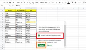
Google Sheets are great for collaborating in real-time. Any individual can easily send an email to the concerned person just with the help of their recipient’s email id. All you have to do is, just insert a plus sign (+), then type the e-mail address (or name) and the recipients will receive an e-mail automatically when you insert your comment. Also, you can make use of the “@” symbol to send an email.
Refer to the steps given below, where you will find an example of how to send an email through google sheet:
- Step 1: Open the google sheet and select the cell where you have to write a mail.
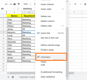
- Step 2: Right-click and select comment from the drop-down menu.
- Step 3: Now either use the “+” or “@” symbol and type the email id as shown in the image given below.
- Step 4: Type the email and click on assign. The email will be sent.
Add Heatmaps Using Conditional Formatting
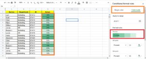
Heatmaps are a great way to highlight important information on your Google sheet. You can use conditional formatting to highlight specific values, outliers, or errors. The function of a colour scale enables you to highlight lower and higher values quickly in your data.
Follow the steps listed below to add heatmaps using conditional formatting.
- Step 1: Click on the “Format” and select “Conditional Formatting” from the drop-down menu.
- Step 2: A new window will open towards the right side of the screen.
- Step 3: Select the “Apply To Range” under “Color Scale“.
- Step 4: Now under format rules, Select the value.
- Step 5: Enter the “Mid Point value, Max point value, Min Point Value“.
- Step 6: Click on “Done“
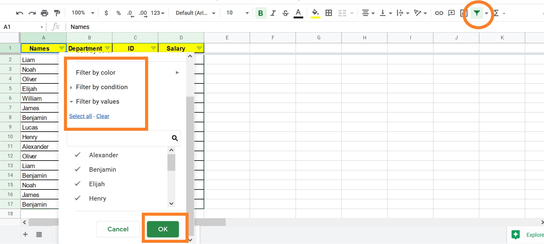
Apply Filters In Google Sheets
You can only display interest rows within the sheet by using filters. This can be helpful if you work with a wider range of data. Follow the steps listed below to apply filters in the sheet.
- Step 1: Select the column on which you will have to apply the filter.
- Step 2: Click on the filter icon as shown in the image below.
- Step 3: Now you will have the option to choose your desired filter by selecting the required dataset and so on.
- Step 4: Also you will have options to filter by colour, values and conditions.
- Step 5: After choosing the desired filter click on “OK“.
- Step 6: The filter will be applied to the sheet.
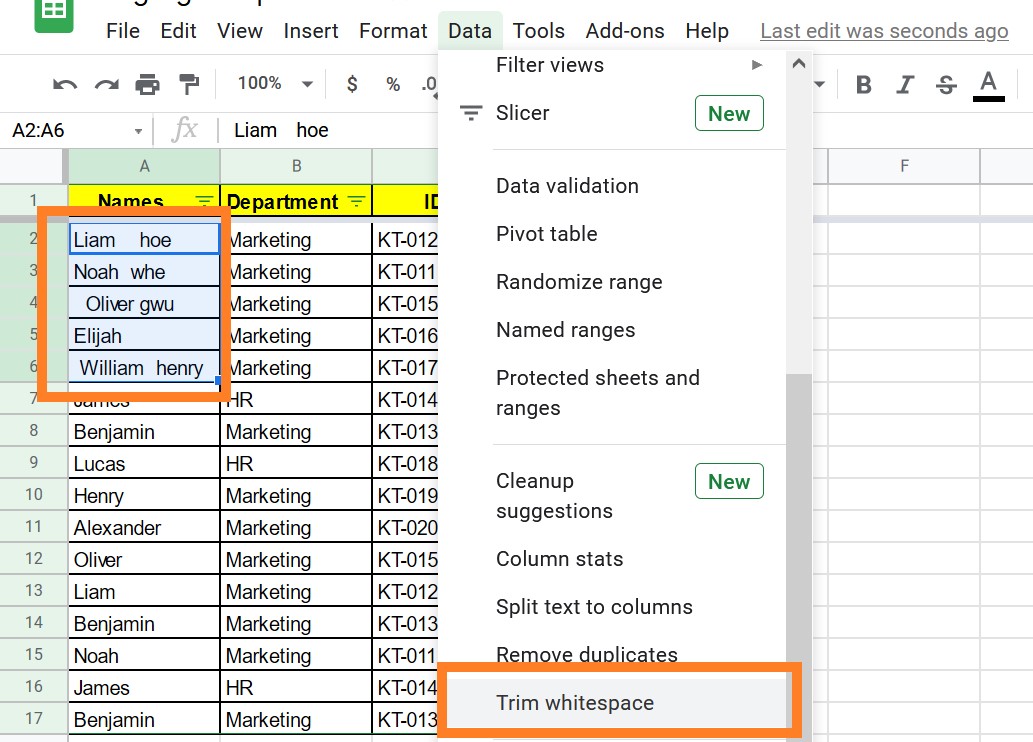
Clean Up Values with CLEAN and TRIM
TRIM function is used to clean or remove from the cell start and from the ends. Follow the steps listed below to make use of the CLEAN and TRIM functions in Google Sheets.
- Step 1: Select the columns where you will have to remove the whitespaces.
- Step 2: Click on the “Data” tab and select “Trim Whitespaces” from the drop-down menu.
- Step 3: Now you will get a message saying that “Trimmed Whitespace from (No) selected rows“.
- Step 4: Click on “OK“.
Another way to trim the whitespace is to simply select the cells and type the formula – “=TRIM(A2)” and the whitespace will be cleaned.
Note: A2 is the cell that we have given here for reference.
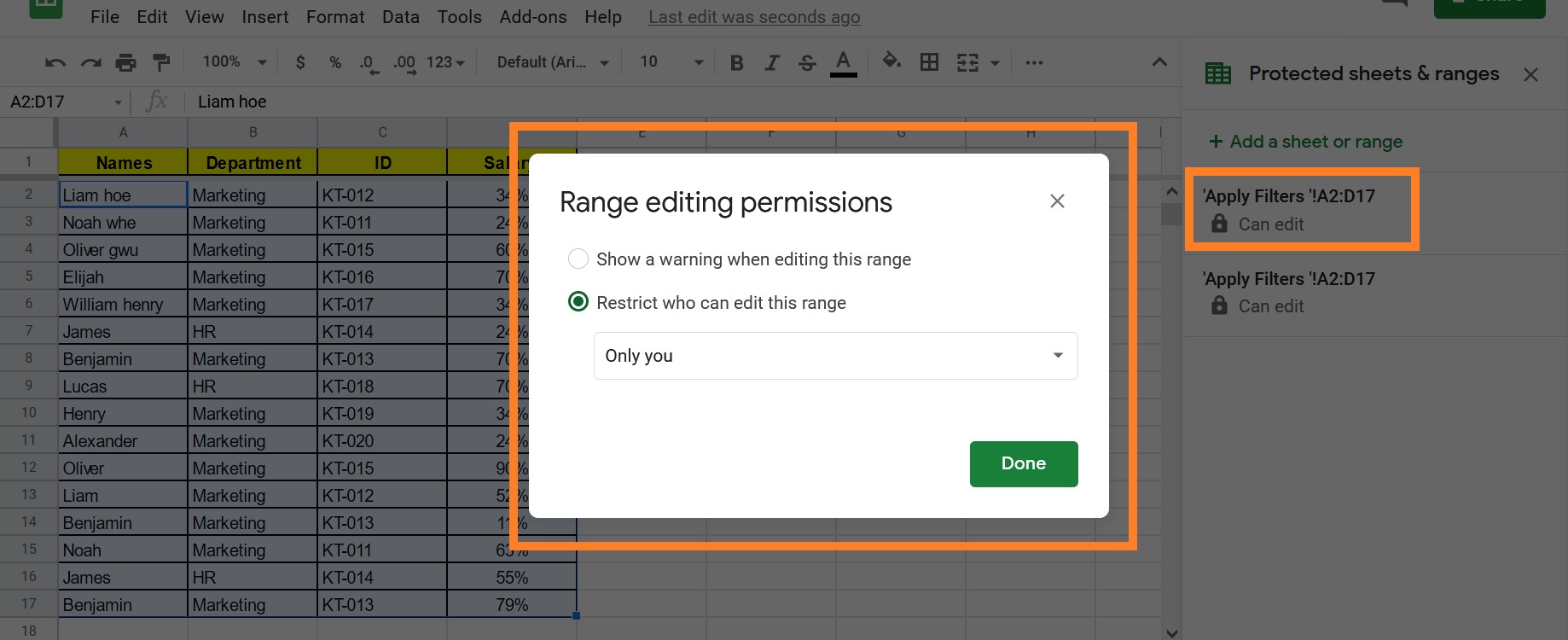
Protect Data in Cells in Google Sheet
You might want to limit data to prevent mistakes if a lot of people work on a sheet. You can also protect sheets and cells so that information is not changed by accident. Follow the steps listed below to protect the data in cells in Google Sheets.
- Step 1: Select the columns and click on the “Data“.
- Step 2: Now, scroll down and select “Protected Sheets and Ranges“.
- Step 3: A new window will open towards the right side of the screen.
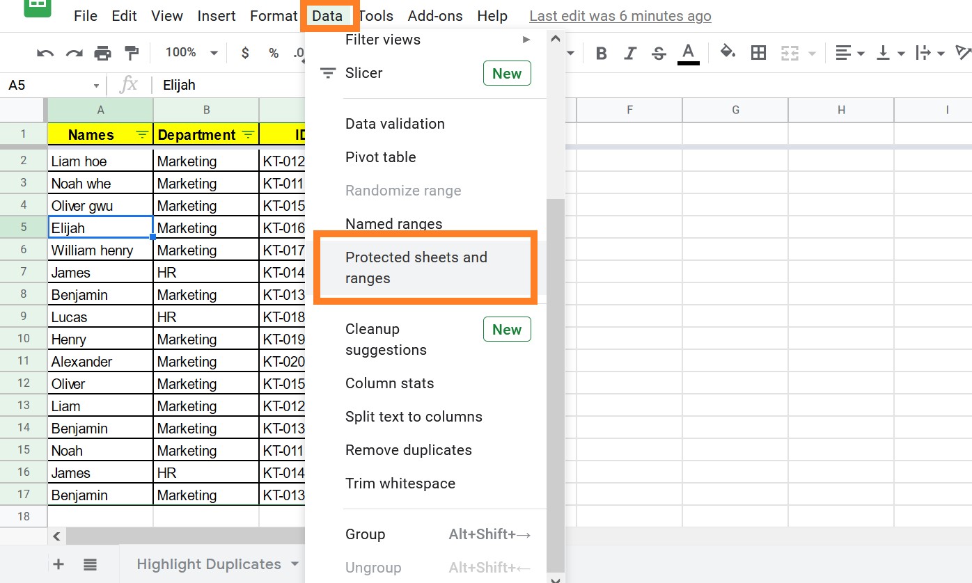
- Step 4: Now select the “Range“.
- Step 5: Click on “Set Permissions“.
- Step 6: Now edit the permissions as per your requirements.
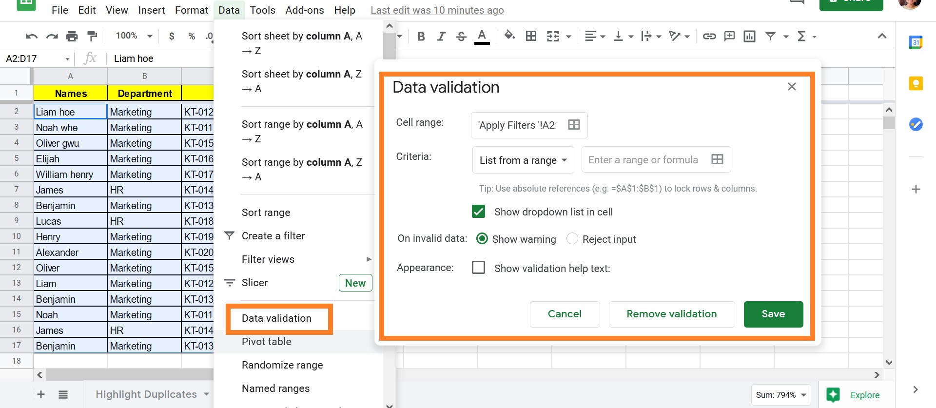
Validate Data in Cells
By applying data validation to your cells on Google sheet, you can ensure that certain cells only contain selected data. For instance, validation can be set to include numbers or even a value in a defined list in certain cells only. A drop-down selector is also made available in the sheet by defining a predefined list of values.
Follow the steps listed below to validate cells using data validation.
- Step 1: Select the cells and click on the “Data” tab.
- Step 2: Now select the “Data Validation” from the drop-down menu.
- Step 3: Validate the selected cells as per your requirements.
- Step 4: Once validation is done, click on “Save“.
Integrate Google Sheet With Google Forms
Although it is one of the most powerful ways to optimise your forms to integrate your Google Form into Google Sheets. You will need to establish a form before you start feeding your Google Sheet information to automatically sync all of your information. It takes only a few minutes to establish your form.
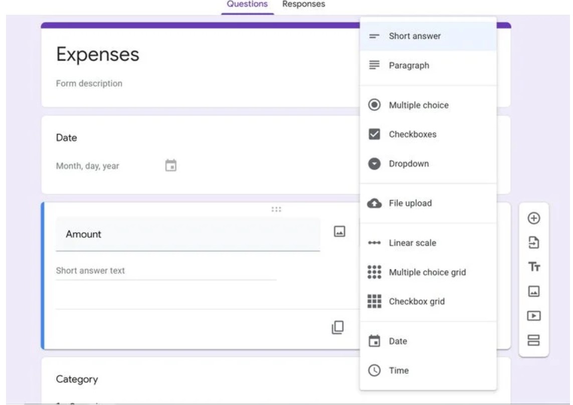
From multiple selections, drop-downs, short answers, long responses, checkboxes, and more, choose different answers.
Follow the steps listed below to integrate Google Sheets with Google Forms.
- Step 1: Click the Responses tab.
- Step 2: Click the Google Sheet icon now.
- Step 3: Choose to create a new spreadsheet.
- Step 4: Enter your sheet name.
- Step 5: Click Create.
Insert a Chart from Google Sheets into a Google Doc
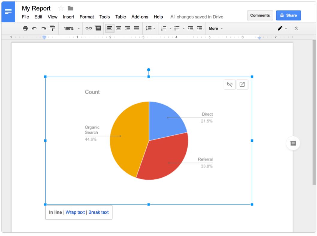
You can insert a chart into Google Docs when you have created a chart inside Google Sheets. Follow the steps listed below to insert a chart from Google Docs to Google Sheets.
- Step 1: Select ‘Insert‘ in the Google document.
- Step 2: Now select “Chart” and hit on “From sheets“.
- Step 3: Now select the “Sheets” from your drive.
- Step 4: Now click on “Select“.
- Step 5: The chart will be displayed on the Google doc.
This saves you much time since you can reflect any modifications made in google sheets by updating the diagram in the document.
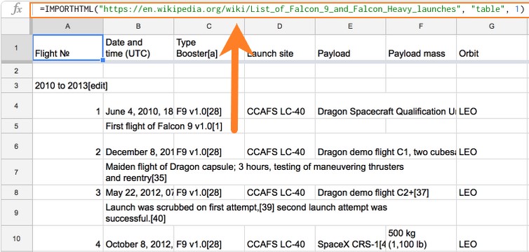
Import Data from a Website or RSS feed
You can import data from websites and RSS feeds via various features. The steps to import data on Google Sheets are explained.
- Step 1: Select the cell where you have to import the data.
- Step 2: Now type the formula “=Import(function type)(URL)”.
- Step 3: Click on “Enter“.
- Step 4: The data will be imported on the sheet.
Various features to import data are:
- ImportHTML tables and lists to import HTML
- ImportFeed to import RSS feed
- ImportData to import a CSV file on the web
- ImportXML to import a customised section of an Xpath webpage.
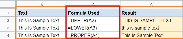
Change Capitalization in Cells
You can use the PROPER function to capitalise on the first letter in each word. This is useful if values are to be cleaned for consistency. Alternatively, the LOWER function can be used to reduce all letters. The steps to change the case are explained below:
- Step 1: Select the cell where you have to make modifications.
- Step 2: Now to capitalize, write the formula “=Upper(Cell Number)“.
- Step 3: Click enter. The word or sentence will be capitalized.
Referto the image below to know the different types of cases used to represent a word.
Also, one can make use of the Add-Ons function in google sheet, to change the case of an word.
Translate Text in Google Sheet
Below is the formula to translate the text,
=GOOLGETRANSLATE(“Text”, “Source Language”, “Destination Language”)
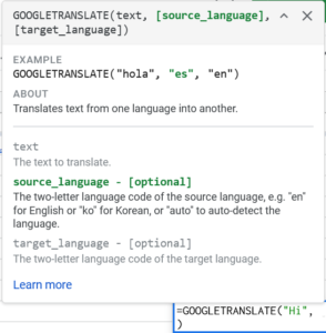
Example:
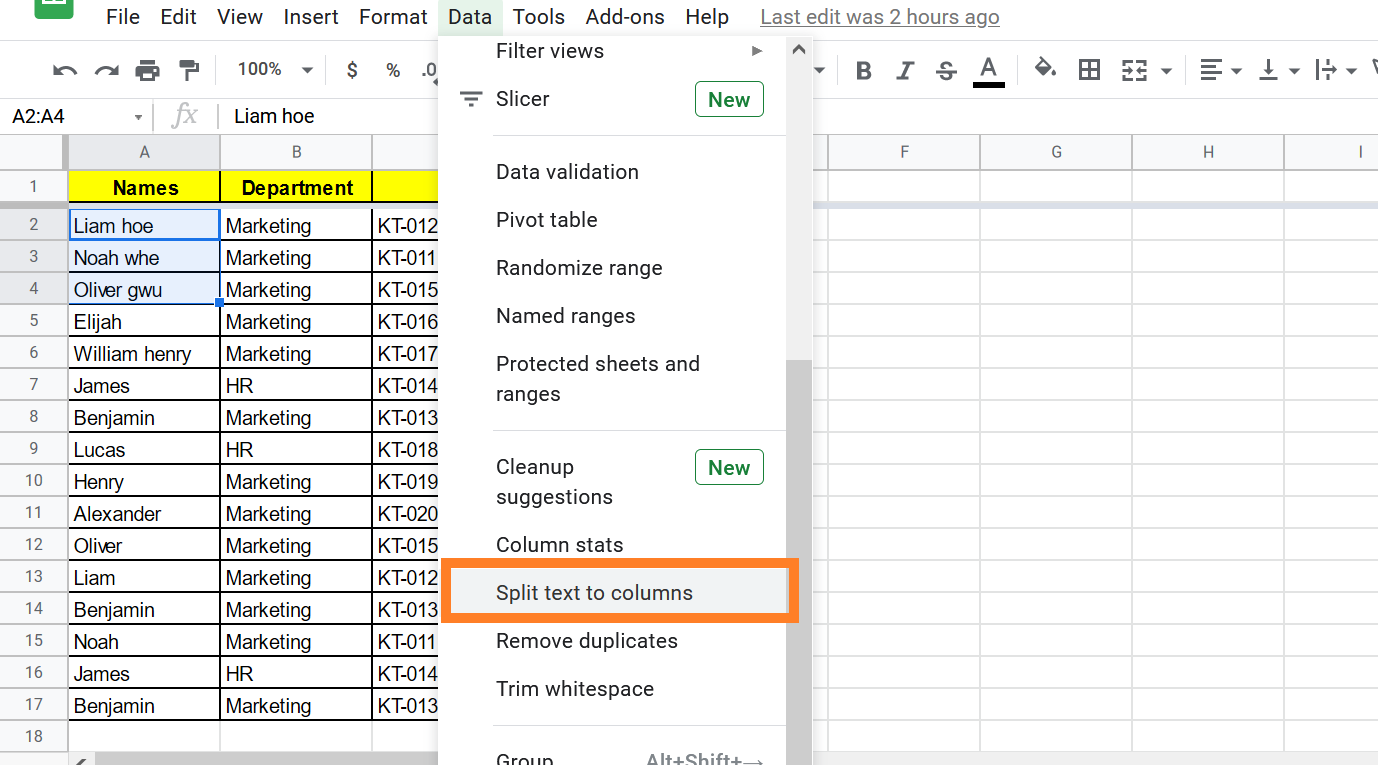
Split Names and Other Data in Google Sheet
These are steps to split the full names into the first name and last name:
- Step 1: Choose the data you would like to divide.
- Step 2: Go to the Data tab.
- Step 3: Click on “Split text to columns“.
- Step 4: It divides the names in the first and last names immediately.
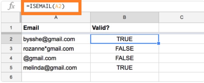
Check for Valid Email Address
You can check it by using Google Sheets if you have a list of e-mails and you want to make certain that they have a valid e-mail address structure. It will not verify that your e-mails are delivered, but it will help identify all rebounding mail addresses (such as ‘@’ or ‘.com’ missing).
- Step 1: Select the cells for which you have to validates the Email.
- Step 2: Enter the formula “=ISEMAIL(Cell Number)“
- Step 3: Click on “Enter“.
- Step 4: The Email Address will be validated with True or False
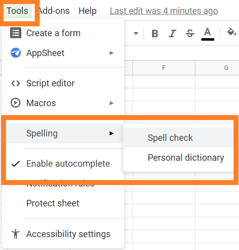
Spell Check in Google Sheet
You can check the word spelling on Google Sheets. Click the Main Menu Tools and then search for Spelling. For a Spell check, click on it. Click on the Spell check and the spelling of words is checked by Google Sheets automatically.
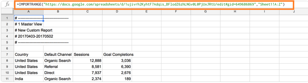
Import Data from Other Sheets
You can simply import data from one sheet to another instead of maintaining data in multiple sheets. This also means that only one place (and not several sheets) needs to update your data, which can save time.
- Open the Google Sheets.
- Enter the formula, “=IMPORTRANGE” in a cell that is empty.
- In parenthesis, in quota marks and separated by a comma* add the following specifications:
- The URL is in sheets of the table.
- The name of the sheet and the cells to be imported are (optional).
- Press Enter.
- Click “Allow” access.
Refer to the image given below for example.
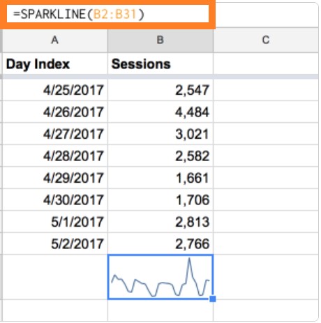
Visualize Data with a Sparkline
In order to quickly see trends in your data, you can easily add sparklines to your sheets.
This may be useful if you compare data or you want to turn your sheet into a dashboard, like comparing metrics, sales and so on. The steps to visualize the data with sparkline are given below:
- Step 1: Select the cells.
- Step 2: Enter the formula “=Sparkline(B2:B31)“
- Step 3: Click on Enter.
You will see a chart showing the trends. Refer to the image given below for reference.
Create QR Codes
Barcodes are a useful way to monitor things, such as checking people for information, conferences or events. And in Google Sheets you can easily create QR codes. All you have to do is, select the cell and enter the formula. The formula to be entered has been provided in the sheet below:
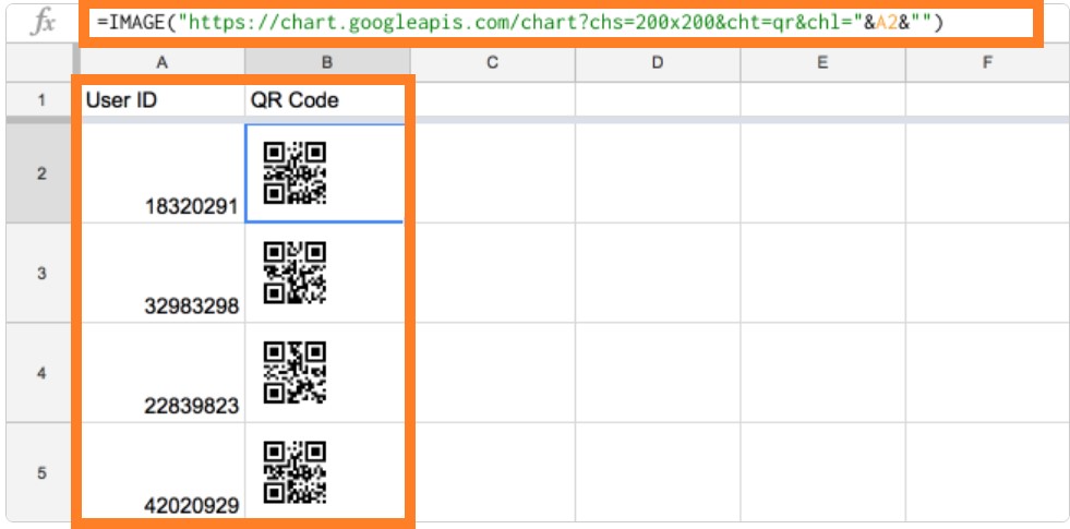
Formula used to create QR code: =IMAGE(“https://chart.googleapis.com/chart?chs=200×200&cht=qr&chl=”&A1&””)
Check if the Cell is Really Blank
The results of a COUNTA() feature that you may use to control the number of cell with existing entries can be misleading characters that do not appear as apostrophic and stray spaces on the table. The solution is to use ISBLANK() to identify which cells have the attributes that offend.
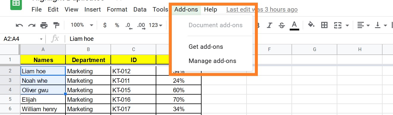
Extend Google Sheets with Add-ons
You can easily add many features to Google Sheets, just by using the “Add-Ons” option. The steps to use add-ons on Google Sheets are explained below.
- Step 1: Click on the “Add-ons” tab.
- Step 2: Click on “Get add-ons“.
- Step 3: You will be displayed with various add-ons tab.
- Step 4: Select the Add-ons and click on “Install for Google Sheets“.
- Step 5: The add-on will be enabled.
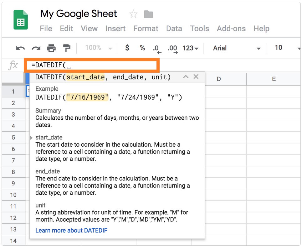
Quickly Learn Formulas
Google Sheets make it easy during work to learn formulas. You will see a handy reference when you begin typing a form that contains important information about the formula you are adding. For example, just start typing the formula = DATEDIF(and you will see this:
Keyboard Shortcuts for Google Sheets
Below provided Google sheets keyboard shortcuts make it easier to perform common actions, like copying and selecting the cells(rows and columns) in the Google sheets:
- Ctrl+C: Copies the selected row/column
- Ctrl+V: Pastes the selected row/column
- Ctrl+X: Cut/Deletes the selected row/column
- Ctrl+Shift+V: Pastes only the value of cell
- Ctrl+Space: Selects the whole column
- Shift+Space: Selects the whole row
- Ctrl+A: Selects entire sheet/cell
- Ctrl+Z: Undo an action
- Ctrl+Y: Redo an action
- Ctrl+F: Find in the sheet/cell
- Ctrl+H: Find and replace in the sheet/cell
- Shift+F11: Insert a new sheet
- Ctrl+Alt+Shift+H: Opens the history of the sheet
Below provided Google sheets keyboard shortcuts will help the user to format the cells easily,
- Ctrl+B: Bold
- Ctrl+I: Italicize
- Ctrl+U: Underline
- Ctrl+Shift+E : Center align
- Ctrl+Shift+L : Left align
- Ctrl+Shift+R : Right align
- Ctrl+; : Insert the Current date
- Alt+Shift+7: Apply the outer border to the selected row/column
- Alt+Shift+6: Removes the outer border for selected row /column
- Ctrl+Shift+1: Format as decimal
- Ctrl+Shift+2: Format as time
- Ctrl+Shift+3: Format as date
- Ctrl+Shift+4: Format as currency
- Ctrl+Shift+5: Format as percentage
- Ctrl+Shift+6: Format as the exponent
- Ctrl+\: Clear formatting from the selected cell
Below provided Google sheets keyboard shortcuts make it easier to move around the spreadsheet easily
- Left/Right/Up/Down Arrow: Move from one cell to another to the left, right, up and down
- Ctrl+Left/Right Arrow: Moves to first or last cell with the data in the row
- Ctrl+Up/Down Arrow: Moves to first or last cell with the data in the column
- Home: Moves to the beginning of a row
- End: Moves to end of the row
- Ctrl+Home: Moves to the beginning of the sheet
- Ctrl+End: Moves to the end of the sheet
- Ctrl+Backspace: Scroll back to the active cell
- Alt+Up/Down Arrow: if you have more than one sheet in the current file, use this shortcut to move to the next or previous sheet
- Alt+Shift+K: Display a list of all sheets
- Ctrl+Alt+Shift+M: Move focus out of the spreadsheet
Below provided Google sheets keyboard shortcuts make it easier to use and find the formulas applied on the sheet.
- Ctrl+~: Shows all formulas in the sheet
- Ctrl+Shift+Enter : Insert an array formula (type “=” first)
- F1: Full or compact formulas help
- F9: Toggle formula result previews
Below provided Google sheets keyboard shortcuts make it easier to Add or Change Rows and Columns eailsy.
- Cmd+D: Duplicate the data from the first column of the selected range down
- Cmd+R: Duplicate the data from the first row of the selected range to the right
- Cmd+Enter: Duplicate the data from the first cell of the selected range into the other cell
- Cmd+Option+9: Hide a row
- Cmd+Shift+9: Unhide a row
- Cmd+Option+0: Hide a column
- Cmd+Shift+0: Unhide a column
- Ctrl+Option+I, then R: Insert the row above
- Ctrl+Option+I, then W: Insert the row below
- Ctrl+Option+I, then C: Insert the columns to the left
- Ctrl+Option+I, then O: Insert the columns to the right
- Ctrl+Option+E, then D: Delete Rows
- Ctrl+Option+E, then E: Delete Columns
Below provided Google sheets keyboard shortcuts make it easier to access the menu easily
- Alt+F: Access the File menu
- Alt+E: Access the Edit menu
- Alt+V: Access the View menu
- Alt+I: Access the Insert menu
- Alt+O: Access the Format menu
- Alt+T: Access the Tools menu
- Alt+H: Access the Help menu
- Alt+A: Access the accessibility menu
- Shift+Right-click: This shows your browser context menu
- Ctrl+Shift+F: Switch to compact mode
Insert Bullets in Google Sheets
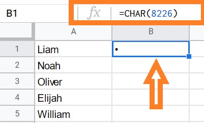
On Google sheets, we don’t have a feature to insert bullets automatically. To insert bullets or number list of Google Spreadsheet, follow the steps listed below:
- Step 1: Choose the cell where you want the bullets to go.
- Step 2: Now type “=CHAR(8226)” in the CHAR function.
- Step 3: On your keyboard, press the “Enter” key.
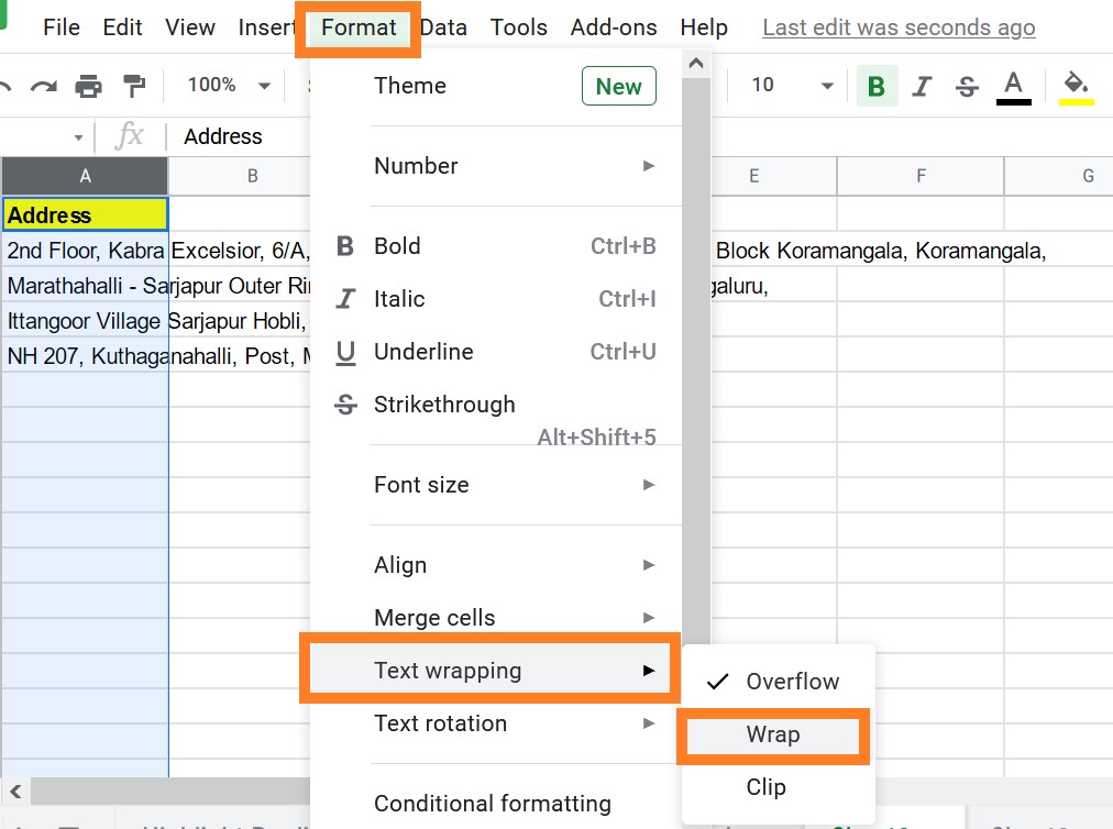
Wrap Text in Google Sheets
- Step 1: Choose the cells you’d like to wrap.
- Step 2: Go to the menu bar and select “Format.”
- Step 3: Go to the section titled “Text Wrapping.”
- Step 4: From the drop-down option, select “Wrap.”
The selected text will be wrapped now.