Have you ever been taught about importing data from one Google Sheet to another Sheet on which you are working on? If yes, then the Google Sheets IMPORTRANGE function is for you. IMPORTRANGE function allows you to import data from another Google Sheets to the desired sheet. All you have to do is to enter the simple formula to import the sheet. In this article, let’s understand how to IMPORT data along with important Google Sheet tips. Read on to find out more.
Table of Contents |
IMPORTRANGE Formula Syntax
The syntax for IMPORT Range function has been explained below:
IMPORTRANGE(spreadsheet_url, range_string)
- spreadsheet url – The URL of the Google Sheets spreadsheet you want to import data from. This URL must be included in double quotations. You may also place the URL in a column and then refer to it from there.
- range string – The cell range you’d like to import. It’s important to note that this must be written in the following format: “[sheet name!]range.” If you wanted to import the cells A1:C10 from a sheet named ABC, then the formula would be “ABC!A1:C10”.
Points to Note:
If you don’t provide a sheet name, the formula will assume you need to import data from the Google Sheets document’s first sheet.
This text can alternatively be placed in a cell and the cell reference is used as the second argument.
Now let’s understand how to import a Google Spreadsheet into the current sheet with the help of an example.
How to Use IMPORTRANGE in Google Sheets?
Let’s consider we have employee name and their salary percentage in sheet 1 and we would like to now import the rating percentage of those employees against their salary. Let’s understand how to do this by using the IMPORTRANGE function in Google Sheets with steps explained below.
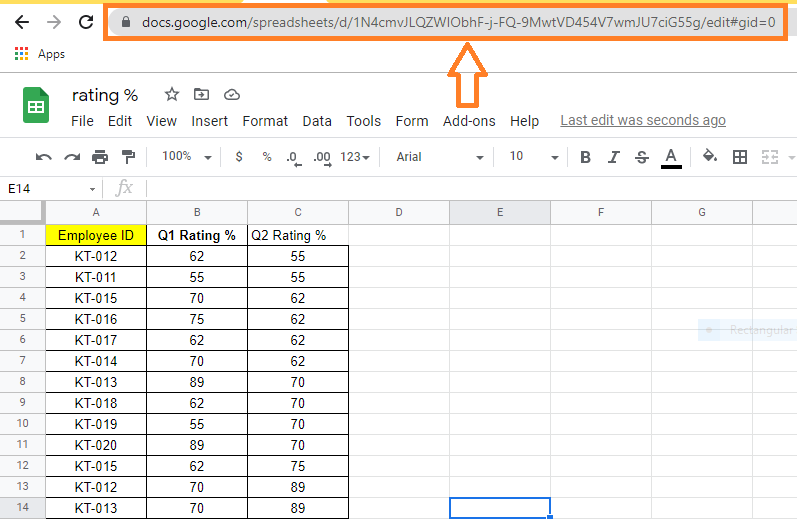
- Step 1: Firstly, open the Google Spreadsheet where you have the rating percentage of the employees. Now copy the part of the URL as shown in the image below.
- Step 2: Now move to the cell where you would like to import the data.
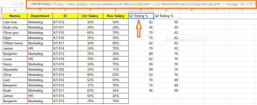
- Step 3: Here, enter the formula as “=IMPORTRANGE(“URL”,”‘Sheet Name’!Cell Range”). In our case the formula is =IMPORTRANGE(“https://docs.google.com/spreadsheets/d/1N4cmvJLQZWIObhF-j-FQ-9MwtVD454V7wmJU7ciG55g/edit#gid=0″,”‘ratings’!B1:C15″).”
- Step 4: Press the “Enter” button. You will see the results.
Points to Note:
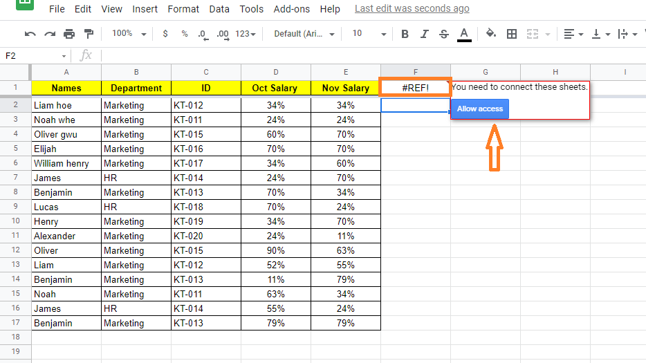
The #REF! error will appear in the sheet when you enter this formula for the first time. When you hover your mouse over the cell, a prompt will appear asking you to ‘Allow access.’ The result will be displayed once you click the blue button. It’s worth noting that this only happens once per URL. It will not ask for access again once you have granted it.
VLOOKUP IMPORTRANGE Google Sheets
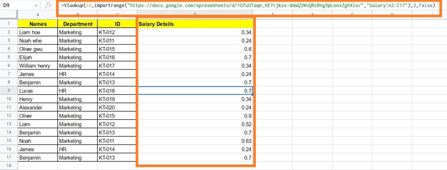
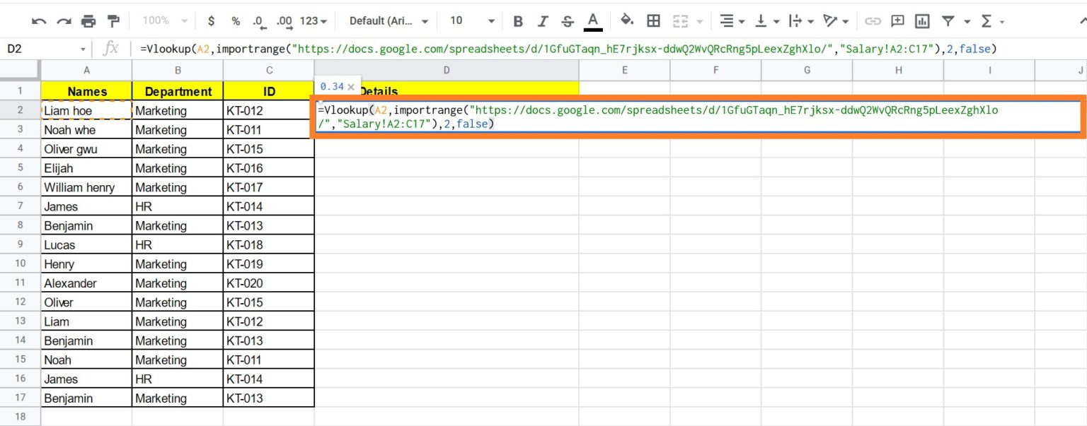
Consider the following example. Now we simply know the employee’s name, ID, and department. Now we must retrieve the employee salary information from the several Google sheets labeled Salary, as shown below.
- How to VLOOKUP from Another Sheet in Google Sheets: Vlookup Between Two Sheets
- How to Sync Data From One Google Sheet to Another Spreadsheet?
- Format Painter in Google Sheets: Copy Paste Text and Images
To VLOOKUP from another worksheet in a separate workbook, follow the steps below.
- Step 1: Choose the cell where you want the data to be called.
- Step 2: Now type “=Vlookup(A2,importrange(“G-Sheet URL”,”Sheet Name!Cell Range”),2,false) into the formula bar. In our case the formula is “=Vlookup(A2,importrange(“https://docs.google.com/spreadsheets/d/1GfuGTaqn hE7rjksxddwQ2WvQRcRng5pLeexZghXlo/,”“Salary!A2:C17”),2,false)“
- Step 3: Press the “Enter” key.
- Step 4: Drag the formula over all of the cells.
- Step 5: The values will be retrieved by the sheet as shown below.