
SUMIFS Function Google Sheets: Google Sheets are widely used in significant organisations for maintaining the data sheets of various financial transactions, employee details, accounts, sales, etc. These include not only data input but also data manipulation such as adding, subtracting, multiplying, and so on as needed.
Hence, instead of manually going on with all the calculations, Google Sheets has come up with certain in-built formulas that will help us achieve the same. One of them is the SUMIFd function. Read on to find out more about the SUMIFS function using Google Sheet tips provided here.
Also Read: Python Interview Questions on User Defined Functions
- How To Use SUM Formula in Google Sheets?
- Using SUMIFs in Google Sheets
- Using SUMIFs Multiple Criteria in Google Sheets
- SUMIFs Google Sheets Date Range
- Using Google Sheets SUMIFs for Multiple Columns
- SUMIFs Array Formula in Google Sheets
- Google Sheets SUMIFs Example
- SUMIFs Function Google Sheets Rules
- SUMIFs Not Working In Google Sheets
- RAMCOCEM Pivot Point Calculator
How To Use the Sum Formula in Google Sheets?
The SUM function in Google Sheets is mainly used to add values. You can use this to add individual values, cell ranges, references, or all three together. The basic syntax of the SUM function is =SUM (cell: cell). Now let’s alter this function accordingly to meet various criteria.
Using Sum To Add Values in a Column
- Step 1: First, select a cell where you wish to calculate and display the sum value.
- Step 2: Next, type =SUM, followed by an open circular bracket, which you can achieve by pressing the Shift and 9 keys together.
- Step 3: Next, click on the first cell of the column from which you wish to start adding the values and drag the pointer to the last cell value to which you want to add.
- Step 4: Here, you will see a formula getting auto-generated in the SUM function cell. Close the circular bracket with Shift+9 and press Enter.
Using SUMIFs in Google Sheets
In other words, the SUMIFs function basically provides you with the sum of a specific set of values by scanning a significant range of data, adding only those that match the given true or false condition, and retrieving the result. The SUMIF function handles one criterion at a time, whereas the SUMIF function can handle multiple criteria at a time. The basic syntax of the SUMIF function is:
=SUMIFS(sumif_range, condition_range1, condition1, condition_range2, condition2, condition_range3, condition3… [condition_range_n, condition_n])
where,
- sumif_range is the cell range containing the values you need to test and add.
- condition_range1 is the range to check for criteria1.
- condition 1 is the criterion that condition_range1 has to satisfy.
- condition_range2, condition2, etc. are the other additional ranges and criteria required for checking.
Google Sheets SUMIFs Example
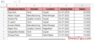
In order to understand the whole scenario of SUMIF better, let’s take an example. Let’s take an employee table, for example, and extract values depending upon certain conditions. The table mentioned below is an employee table that has the details of eight employees. The details mentioned include the employee name, domain of work, location, date of joining, and salary.
Using SUMIFs Multiple Criteria in Google Sheets
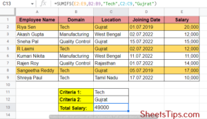
The SUMIF function works with a single condition, whereas the SUMIFs function helps us work with multiple conditions or criteria. To understand this better, let’s consider the table mentioned above and try to calculate the sum of the total salary of all the employees who are from and work in the domain.
Criteria mentioned: Location= Gujrat, Domain= Tech.
So the parameters required for the SUMIFS function here are:
- sum_range will be the values within E2:E9 depicting the salary column.
- criteria_range1 will be the values within B2:B9 depicting the domain column.
- criteria1 will be “Tech” because we want to extract the cells where department = “Tech“.
- criteria_range2 will be the values within C2:C9 depicting the location column.
- criteria2 will be “Gujrat” because we want to extract the cells where location = “Gujrat“.
Hence, the final formula here is: =SUMIFS(E2:E9,B2:B9,”Tech”,C2:C9,”Gujrat”).
SUMIFs Google Sheets Date Range
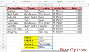
Now, let us consider the SUMIF function using a date range as a condition. For example, we want to extract the sum of all those employees whose date of joining is before July 7th, 2022. So, here we need to add a new date condition along with location and domain, that is < 07.07.2022. Let’s see the implementation now:
The added criteria syntax will be D2: D9, which is the joining date as the third criteria range for values < 07.07.2022. The final formula is:
=SUMIFS(E2:E9,B2:B9,”Tech”,C2:C9,”Gujrat”,D2:D9,”<01/01/2020″)
Using Google Sheets SUMIFs for Multiple Columns
Using SUMIFs for multiple columns is not allowed in Google Sheets. You can use SUMIFs to achieve a result in one column after checking multiple criteria because SUMIF can handle only one condition at a time. However, let’s see an example where you can use the OR logic in SUMIFs to add two calculations together:
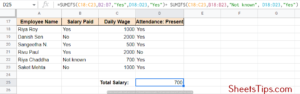
Let’s find out if you have paid any employees incorrectly from your payroll table. Here we need to copy the same calculation twice, but this time with one calculation using “Yes” or “No” as criteria :
=SUMIFS(C19: C24,B19: B24,”Yes”,D19: D24,”Yes”)+ SUMIFS(C19: C24, B19: B724,”Not known”, D19: D24,”Yes”)
SUMIFs Array Formula in Google Sheets
The SUMIFs function cannot be used directly with arrays because it deals with multiple criteria and doesn’t expand a particular one from the array. However, there are two methods we can follow here. They are given below. Let’s take the following table as an example to understand better:
- Using the SUMIF function. This can be a bit tricky but can expand your array output thoroughly by combining ranges with corresponding criteria. The formula used should be: = ArrayFormula(sumif ( F2: F17& G2: G17, H2: H4& I2: I4, D2: D17))
SUMIFs Function Google Sheets Rules
Every Microsoft Excel function comes with its given set of rules. Here are some of the things you need to keep in your mind while using the SUMIFS function in calculations:
- Operators can be used with SUMIFS Functions.
- The additional ranges need to have matching rows and columns as per the sum_range.
- While SUMIFS is for multiple conditions, SUMIF is for single condition calculations where text, dates, and numbers can be used as criteria.
- We can use wild card functions like (?,*) also in SUMIF and SUMIFs calculations.
- We cannot use ARRAYs directly with SUMIFS functions but can be used with SUMIF.
- The Text strings need to be in quotes but cell references should not.
SUMIF Not Working in Google Sheets
SUMIF works with two ranges at a time. Hence, sometimes it may show errors or wrong results if you happen to give the wrong formula or multiple criteria at a time. You can use the F9 key in such a situation to recalculate the sheet and enter formulas manually. Make sure you stick specifically to the formula =SUMIF( condition_range, condition, sum_range) while using SUMIF and try to avoid uneven data format.