
Calculate Days Between Two Dates in Google Sheets: Handling extensive data sheets with multiple dates and time combinations is very common these days. Calculating the number of days between two dates by subtracting in Google Sheets is possible for small data worksheets. But for huge lumps of data, calculating days between months will be time-consuming, prone to errors, and tedious.
But, thanks to Google Sheets, because has provided us with dedicated formulas to help us achieve this in no time. Google Sheets allow us to work with calendar functions, dates, timesheets, etc. for unlimited volumes of data. So let’s see what these amazing Google Sheet tips are in detail, so stay tuned till the end.
- How To Calculate Number of Days Between Two Dates in Google Sheets?
- How To Calculate Working Days Between Two Dates?
- Steps To Count Days Between Dates Using the Days Function
- Compare Days Between Dates Using the Datedif Function Google Sheets
- How To Compare Dates in Google Sheets Using the minus Function?
- How To Calculate Weeks Between Two Dates Google Sheets?
- How To Calculate Months Between Two Dates Google Sheets?
- FAQS
How To Calculate Number of Days Between Two Dates in Google Sheets?
While handling a project, let’s say you encounter the start date and end date of a particular series of entries and want to calculate the total number of days between these two dates. You can easily do this by subtracting the start date from the end date since dates are all about numbers too. Let’s see the below example to understand this better.
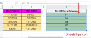
Say, for example, you have the start date and end date in columns A and B respectively, and aim to find out and print the total number of days between in another cell. If the start date and end date are in columns B1 and B2, type the formula B2-B1 on your output cell reference and hit Enter. If you want to enter the start date too just add one to this formula or B2-B1+1.
How To Calculate Working Days Between Two Dates?
While handling large amounts of employee data like payroll, attendance, etc., you do get start and end dates to calculate the total number of days between. But in such situations, you only have to consider work days and exclude weekends.
Well, counting days just by subtracting the start date from the end date in these scenarios will not be that straightforward, so you will need to incorporate a whole different formula for that.
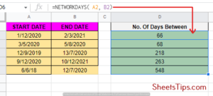
Let’s take this data set as an example where you need to calculate the total number of working days between the dates mentioned in B1 and B2. Select the cell where you want to display the output and put the formula =NETWORKDAYS( B1, B2).
The NETWORK function takes the start date and end date as parameters and generates output based on the networking days in between, excluding Saturdays and Sundays.
But, this formula will be insufficient because we have public holidays too, which are not considered working days either. Also, some companies have their own rules for weeks off.
Some may give you a Saturday-Sunday week off, while another may give you a Monday-Wednesday off, and so on. So the formula here has to be a bit different. Say, your company has provided you with a work calendar like the one mentioned below that has a specified column for company holidays.
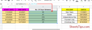
Say, you have your holiday column at E2: E12. Just by upgrading your NETWORKDAYS formula a little bit, you can make it ignore these cells that include company holidays while calculating the work days.
Select the cell where you want to show this result and put the formula =NETWORKDAYS (B1, B2, E2: E12). Another amazing feature about this is that NETWORKDAYS makes sure to not remove a day twice if it is a weekend as well as a public holiday.
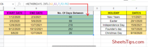
To calculate workdays for companies where weekends are not Saturday and Sunday, the INTL function will come into play. That stands for International. The format of the formula is =NETWORKDAYS.INTL, which takes the start date, end date, and holidays as parameters, along with allowing us to specify the weekend or any two consecutive days.
In the following sample table, you will see a holiday and weekend table. Type the formula =NETWORKDAYS.INTL ( B1, B2, 7,E2,E12 ) into the result cell. When B1 is the start date, B2 is the end date, and E2:E12 is the holiday date column, then 7 is to specify the weekend days where you want this formula to work. To know why follow the table below.
So, based on this if you only want Sunday to be considered a weekend use 11 as the third parameter in the NETWORKDAYS.INTL function.
Steps To Count Days Between Dates Using the Days Function
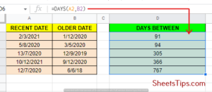
The DAYS function is one of the easiest ways to calculate the number of days between dates in Google Sheets if you don’t want additional operations such as excluding weekends, holidays, etc. The syntax of the formula you need to follow is =DAYS (“end_date,” “start_date”). You can either type the dates manually or can also use cell references. Follow the steps below:
Step 1: Select an empty cell where you want to display the result and type =DAYS and hit Enter.
Step 2: Next, type the dates or select the cell references with the dates along with a comma in between and press Enter. For manual data entry, make sure you don’t forget to use quotation marks (” “) around the dates.
In the sample table below, in cell D2, if we type the dates manually or use cell references, in both cases we will yield the same result.
Compare Days Between Dates Using the Datedif Function Google Sheets
The DATEDIF function is quite similar to the DAYS function, but the main difference is that you need to provide a unit for the syntax along with interchanging the positions of the start_date and end_date. The syntax of the formula is: DATEDIF( start_date, end_date, unit).
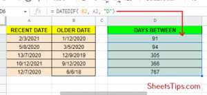
In the above example table, input the formula on the result cell along with the start_date, end_date, and a unit corresponding with our condition for the DATEDIF function. We have used “D” here to notify Google Sheets that we want the results in days. The DATEDIF function unit list that we use as shortcuts is as follows:
- Y calculates the result in years.
- M calculates the result in months.
- MD refers to the difference between dates while ignoring the months and years.
- YM refers to the months in between dates while ignoring the years and days.
- YD returns the days in between dates while including the months and ignoring the years.
How To Compare Dates in Google Sheets Using the minus Function?
The MINUS function in Google Sheets can be used to calculate date differences with a formula syntax of =MINUS(Value1, Value2). To work with dates, the formula will be =MINUS(end_date, start_date). The following example shows the result of the MINUS function on the same table we used the DAYS function on.
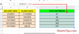
Although we get the same results, it is always recommended to use the DAYS function because it is easier to enter the dates from the columns in Google Sheets and will also make your spreadsheet portable to Microsoft Excel. The MINUS function doesn’t work for Microsoft Excel.
How To Calculate Weeks Between Two Dates Google Sheets?
If you want to count the total number of whole weeks between two dates, you can just simply subtract the start date from the end date and then divide the result by 7. To use the DATEDIF function, follow the steps mentioned below as per our example:
- Step 1: Select any blank cell to display the output and put the formula =(DATEDIF(A2, B2, “D”)/7) =(B2-A2)/7, where A2 is the start date cell and B2 is the end date cell.
- Step 2: Next, drag the fill handle plus button down to fill the entire column with this formula, and you will see the output as weeks in decimal numbers.
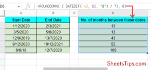
To get the total number of full weeks between the two dates, use the formula =ROUNDDOWN( ( DATEDIF( A2, B2, “d”)/7), 0)= INT((B2-A2)/7).
How To Calculate Months Between Two Dates Google Sheets?
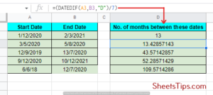
To count and display the total number of months between two given dates, the best option is to use the DATEDIF function again. From the example below, follow these steps:
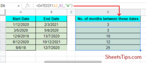
- Step 1: Select any blank cell where you want to print the result and put the formula =DATEDIF (A2,B2,,”m”) where A2 is the start date cell and B2 is the end date cell.
- Step 2: Next, drag the fill handle + button down again to fill this formula across the entire column. The final result you see is the number of total completed months between the given start and end dates.
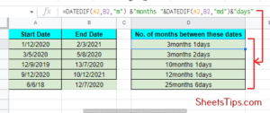
- Step 3:To get the total number of full months and days between the two dates, use the formula =DATEDIF(A2,B2,”m”) & “months” &DATEDIF(A2,B2,”md”)&”days”
FAQs on How To Calculate Days Between Two Dates
1. How do I calculate the number of days between two dates?
If you want to calculate the number of days between two dates, subtract the start date from the end date. If it crosses years, then calculate the number of full years. If it crosses months, then calculate the number of months. You can also use the =DAYS (“end_date,” “start_date”) function.
2. How do I count down the days in Google Sheets?
To create a countdown timer in Google Sheets, use the NOW() function to calculate the number of days, hours, and minutes. For days, use =INT (A2-NOW()), for hours, use =HOUR (A2-NOW()), and for minutes, use =MINUTE (A2-NOW()).
Also Read: Java Program to Print Series 7 14 21 28 35 42 …N
Must Read: