Calculated Fields are very useful when it comes to summarising the data in Google Sheet Pivot tables. The main purpose of Calculated Fields is that it allows you to process your data in order to create more tailored Pivot table results. With the help of Custom formulas, one can present summary metrics in the Pivot table using calculated fields without making any changes in the actual dataset. In this article, let us understand how to add and use the Calculated Fields with the Google Sheet tips provided on this page. Read on to find more.
Also Read: Mining Engineering Notes
Table of Contents |

How to Create Pivot Tables in Google Sheets?
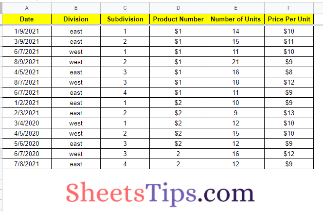
Let us consider the following dataset which represents the sales data of each division.
- How to Group by Month in Pivot Table in Google Sheets (With Examples)
- How to Refresh Pivot Table in Google Sheets: 3 Ways to Refresh Pivot Tables
- How to Insert a Pivot Table in Google Sheets? (Create/Edit/Customize Pivot Tables)
Now follow the steps listed below to create a Pivot table for the above dataset.
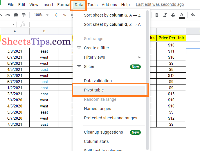
- Step 1: Click on the Data tab from the menubar.
- Step 2: Now choose “Pivot Table” from the drop-down menu.
- Step 3: You should now see a window asking whether you want to place your pivot table into an existing sheet or create a new one. Choose your preferred option. It’s always advisable to make one in a new sheet for clarity.
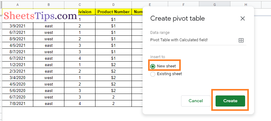
- Step 4: Click on the “Create” button.
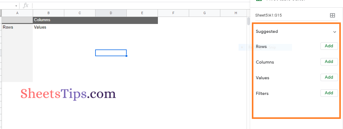
- Step 5: Now the Pivot table will be created in the new sheet. The Pivot table will look like the following image at this stage.
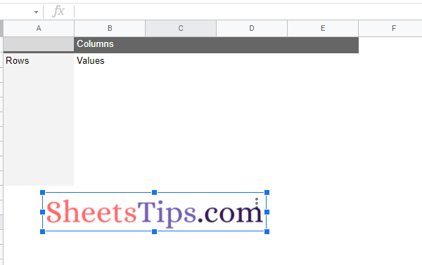
- Step 6: A grid of ‘Rows, Columns, and Values‘ should be displayed. You may now begin populating your pivot table with the information you desire. A Pivot Table Editor should appear on the right side of the window. This will assist you in determining what should be included in your pivot table.
How to Add Calculated Fields in Google Sheet?
Now let us understand how to add the calculated fields using the SUM function in Google Sheets with the help of the steps given below:
- Step 1: Select the pivot table by clicking on it.
- Step 2: Click Add next to “Values” on the side panel.
- Step 3: Select the Calculated field box from the drop-down menu.
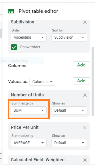
- Step 4: To use SUM to calculate a value, click SUM next to “Summarize by.“
- Step 5: To use a custom formula to calculate a value, follow these steps: Enter a formula in the field that displays. In our case the formula is =SUM(arrayformula(‘Number of Units’*’Price Per Unit’))/sum(‘Number of Units’)
- Step 7: Then click Custom next to “Summarize by.“
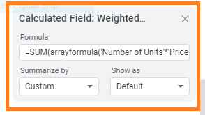
- Step 8: Click Add in the bottom right corner to add a new column.
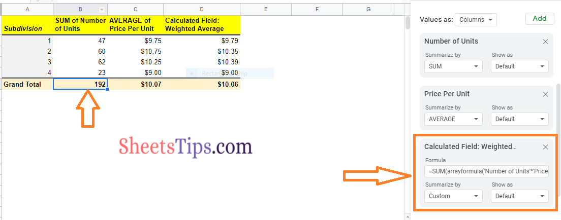
Now you can see the results as shown below:
Points to Note About Calculated Fields in Google Sheets
Pivot tables with calculated fields have a lot more flexibility and versatility. It does, however, have some restrictions. As a result, some considerations must be made while creating calculated fields.
- Only cells from your original dataset are referenced in your computed field calculations. They can’t refer to the totals or subtotals in the pivot table.
- In the calculated field formulas, you must use the field names from your dataset. Individual cells cannot be referred to by their address or cell names.
- It’s critical that you use the correct variable name for each field in your formula. If your field name has more than one word with spaces between them, you must use single quotes to surround the variable name in the calculated field’s formula.
Must Read: