
Spreadsheets are an excellent tool for working with data. They assist you in organizing your data so that you can gain useful information and insight from it. Google Sheets includes the Pivot table feature, which makes data analysis even more powerful.
If you are new to the Pivot table, then this article will help you to understand everything about Pivot tables with the help of Google Sheet tips provided on this page. Read on to find more.
Table of Contents |
What are Pivot Tables in Google Sheets?
Pivot tables aid in the summarization of data, the discovery of patterns, and the reorganization of information. You can either add pivot tables based on Google Sheets suggestions or create them manually. You can add and move data, add a filter, drill down to see details about a calculation, group data, and more after you create a pivot table.
How to Add Pivot Table From Google Sheets Suggestion?
Follow the steps as listed below to add a pivot table with the help of Google Sheets suggestion:
- Step 1: Open the Google Spreadsheet where you want to add a pivot table.
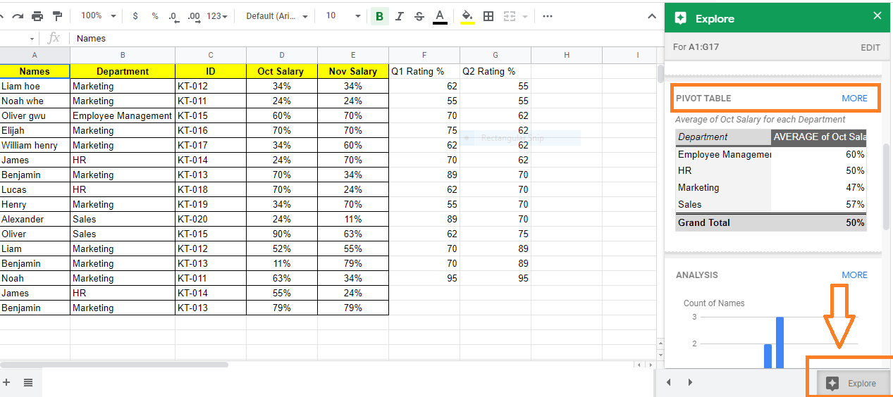
- Step 2: Now at the bottom of the Google Spreadsheet, click on the “Explore” button. Alternatively, you can also use the Keyboard shortcut (Alt+Shift+X) to enable the Explore button.
- Step 3: The explore menu will open up on the screen. Now click on the Pivot Tables shown up in the window.
- Step 4: Now the preview link of the Pivot table will be shown on the screen. Click on “Insert Pivot Table“.
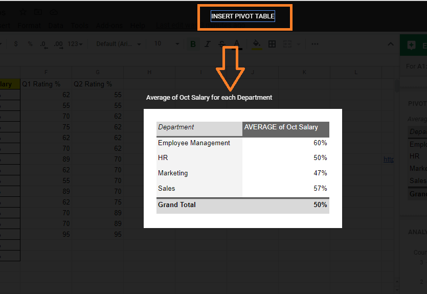
- Step 5: That’s it, the new Pivot table is added to the sheet.
Note: If a Pivot table is not applicable to your data, the pivot table wouldn’t be generated on the sheet. In order to insert the Pivot table in Google Sheets, the data you use should be organized into columns, with a header for each column.
- Auto Suggested Pivot Chart in Google Sheets: Parameters for Creating Pivot Table Using Explore
- How to Make a Line Chart in Google Sheets: Setup/Edit/Customize Line Graph
- How to Make a Histogram in Google Sheets: Create/Delete/Customize Histogram Graph
How to Create Pivot Table Manually in Google Sheets?
Follow the steps as listed below to create a Pivot table manually in Google Sheets:
- Step 1: Open the Google Spreadsheet.
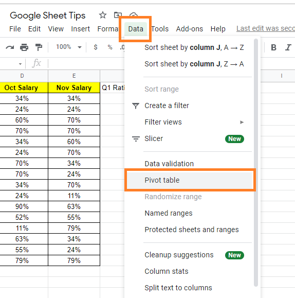
- Step 2: Click on the Data Tab and select Pivot table from the drop-down menu.
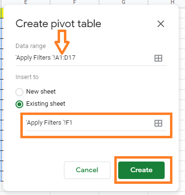
- Step 3: Now a window will appear on the screen. In this window choose Data Range.
- Step 4: In the same window, there will be two options named “Insert To“. Here select New Sheet to create a Pivot table in the new sheet or select Existing Sheet to create the pivot table in the existing sheet.
- Step 5: Now click on the “Create” button.
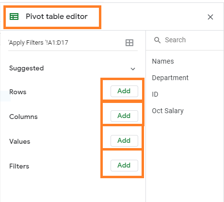
- Step 6: Enter the cell range where the Pivot table should be created. Now the Pivot table editor will open towards the right side of the screen. With the help of the Pivot table editor, you can customize your table.
How to Edit or Customize Pivot Table in Google Sheets?
Firstly in order to edit the Pivot table, click anywhere on the table. The Pivot table editor window will open towards the right side of the screen. Now you will be provided with a list of the following options with the help of which you can customize the Pivot tables in Google Sheets.
To Add Data: In the Pivot table editor, you will see 4 options namely rows, columns, filter, values. Just click on the Add button below each section to add the data.
To Change Row/Column Name: Double click the row or the column to change the name.
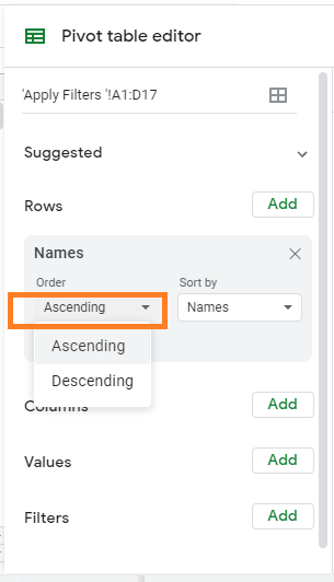
To Change Sort Order/Column: Click the Down arrow under Rows or Columns. Select the option or item under Order or Sort by. This will sort the data.
To Change the Data Range: Select the data range and enter the new range.
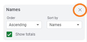
To Delete Data: To delete the data, click on the “X” icon as shown below. This will delete the data which was created earlier.
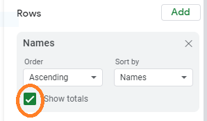
To Show Totals: Check the Show Totals box under Rows or Columns.
To Show Values as Percentages: Under Values, click the Down arrow, then select a percentage option under Show as.
How to Hide Data With Filter in Pivot Table?
We can hide data with filters in the Pivot table by following the steps as listed below:
- Step 1: Click on the Pivot table and the Pivot table editor will open towards the right side of the screen.
- Step 2: Now move the Filter section.
- Step 3: Click on the “Add” button. Select the column or row which needs to be included in the Filter.
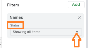
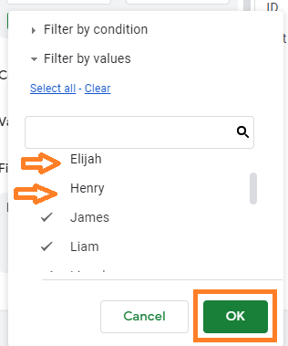
- Step 4: Now under the “Status” section, select the list of rows or columns which need to be hidden.
- Step 5: Click on the “Ok” button.
The selected row or column would be hidden.