A Pivot Table in Google Sheets is a function for summarising, sorting, reorganizing, grouping, counting, totaling, or averaging data in a table. It allows us to change rows into columns and columns into rows. It lets you organize your data by any field (column) and perform advanced calculations on it.
Also with the help of the Google Sheets Pivot table, we can group the data by week, month, year, and even a day. In this article, let’s understand how to group Pivot tables with the help of Google Sheet tips provided on this page. Read on to find out more.
Table of Contents |
How to Group by Month in Google Sheets Pivot Table?
In order to group by month in the Google Sheets Pivot table, make sure your dataset is having the data values which are mentioned in proper date format.
Now let’s consider the following example where we can group by month in the Google Sheets Pivot table.
How to Create Date Values In Google Sheet?
Suppose if your dataset doesn’t have proper date values, then you can use the following steps to create the proper DATE format in Google Sheets.
- Step 1: Select the Date column, where you can create a proper DATE format.
- Step 2: Now click on the “Format” from the menubar and select “Number” from the drop-down menu.
- Step 3: The Number sub menu will be displayed on the screen. Choose “Date” from the sub-menu.
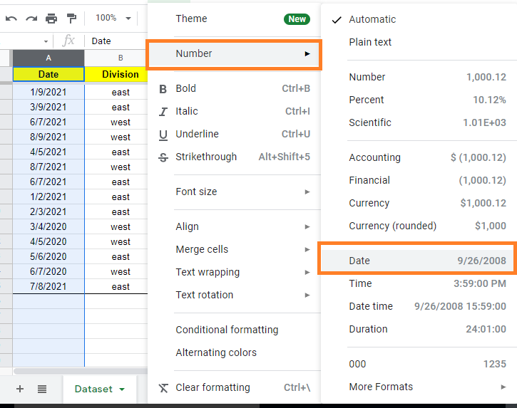
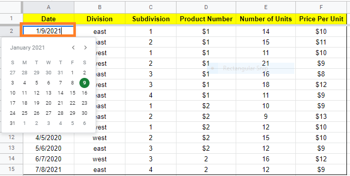
The selected columns will now have Date Values in the form of Google Sheets DATE format.
How to Create Pivot Table to Group Date-wise?
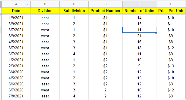
Consider the following dataset. Now follow the steps listed below to create a pivot table and group the date-wise.
- Step 1: Open the Google Sheet.
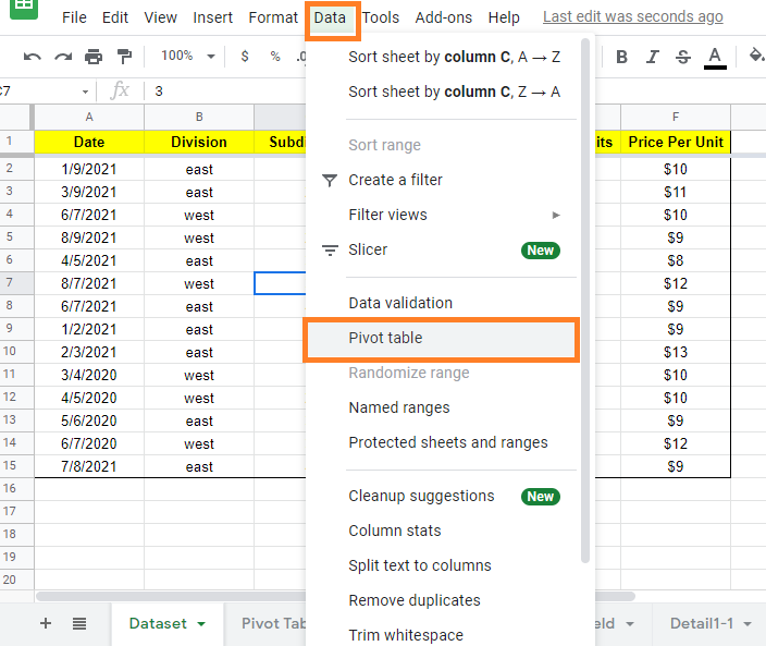
- Step 2: Click on the “Data” from the menubar and select “Pivot Table” from the drop-down menu.
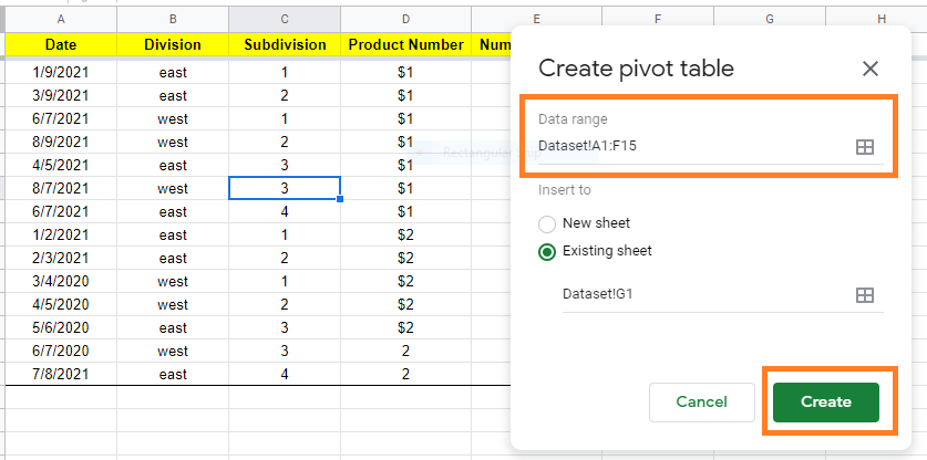
- Step 3: Now the Pivot table box will appear on the screen. Here choose the data range and check the box where you would like to create the pivot table.
- Step 4: Once the necessary actions are taken, just click on the “Create” button.
- Step 5: This will create the Pivot table in the specified place. Now click on the Pivot table. The Pivot table editor will open on the screen.
- Step 6: Under the Pivot table editor, start adding your data by clicking the “Add” button under column, row, filter, values.
- Step 7: As soon you add the data, click on the “Add” button and choose “Date“.
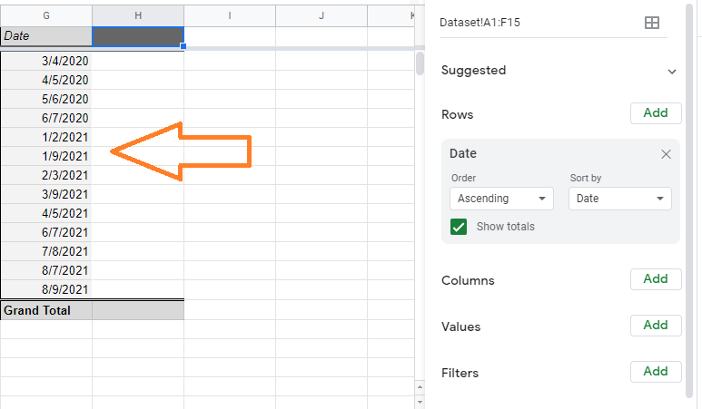
This will order the data date-wise as shown below.
- Google Sheets QUERY Function Explained With Examples
- How to Group Columns in Google Sheets? (Group Multiple Columns, Collapse)
- How to Make a Histogram in Google Sheets: Create/Delete/Customize Histogram Graph
Grouping Google Sheets Pivot Tables by Month
Follow the steps listed below to group the Google Sheets pivot tables by month.
- Step 1: In the previous section, we grouped the Pivot table date-wise.
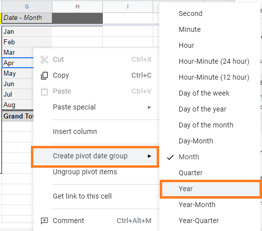
- Step 2: Now right-click on any of the dates under the “Date” column.
- Step 3: The context menu will open up on the screen. Now select “Create Pivot table date group” from the context menu.
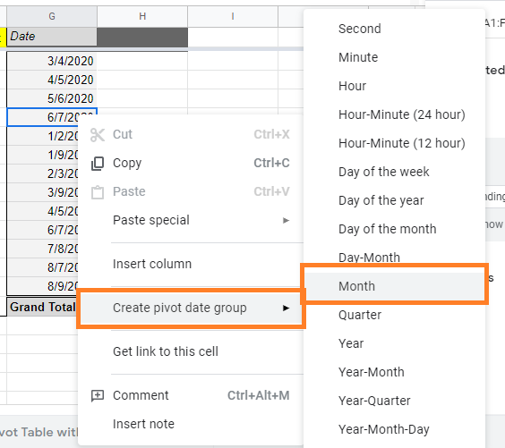
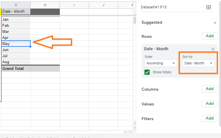
- Step 4: Now another sub-menu will open on the screen. Here you will be provided with so many options. Choose “Month” in this sub-menu.
- Step 5: This will group the columns month-wise as shown below.
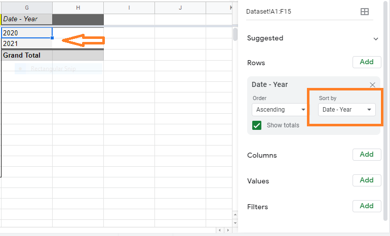
To group Pivot Table by Year, right-click on the Date column and select “Year” from the context menu.
When you group pivot table by year, the result will be as follows: