
If you want to delete every other row in Google Sheets manually, it is a time-consuming process. In order to save your time, you can use ISEVEN or MOD function, with the help of which you can delete every other row, Nth row, third row, and so on.
In this article, let’s understand how to delete alternative rows with the help of Google Sheet tips provided on this page. Read on to find more.
Table of Contents |
Delete Every Other Row using in Google Sheets using Filter Icon
Follow the steps as listed below to delete every other row in Goole Sheets using the Filter icon:
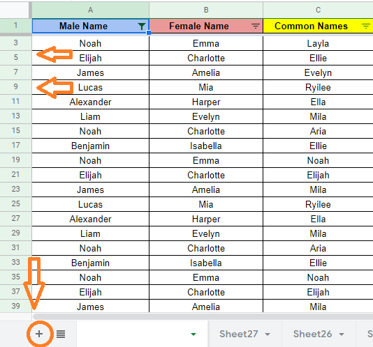
- Step 1: Select the columns where you would like to delete every other in Google Sheets.
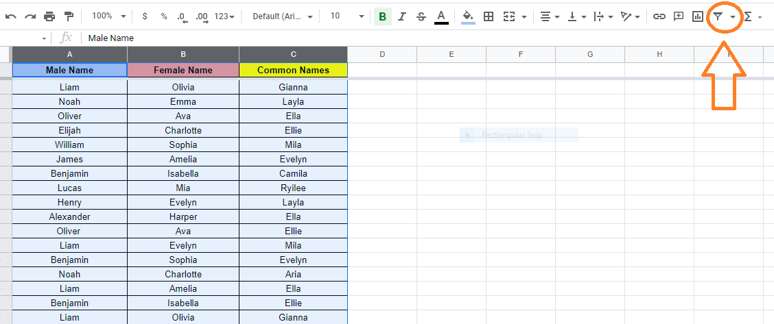
- Step 2: Apply the Filter using “Filter Icon” from the toolbar.
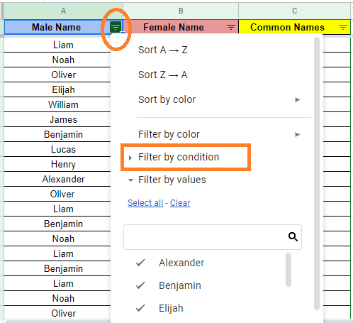
- Step 3: Now click on the Filter icon in the column header and select “Filter by Condition” from the drop-down menu.
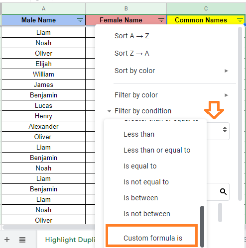
- Step 4: Select “Custom Formula” in the empty field.
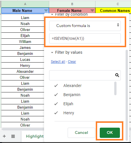
- Step 5: Now enter the formula as “=ISEVEN(row(A1))“.
- Step 6: Click on the “Ok” button. You will see the results.
- Step 7: Now select all of the fields on the worksheet (Ctrl+A on a PC, CMD+A on a Mac), “Copy” the values (Ctrl+C on a PC, CMA+C on a Mac), and then click the “+” icon to make a new worksheet/page.
- Step 8: Paste the visible contents from the previous worksheet/page into the new worksheet/page (Ctrl+V for PC, CMD+V for Mac) by clicking on cell A1 on the new worksheet/page. Every other row in the worksheet has now been erased.
How to Delete Nth Row in Google Sheets?
Deleting every other row in Google Sheets is quite easy. But if you want to delete the 3rd row, 5th row, 6th row, and so on, then you can use the MOD function. Though the MOD function is a bit tricky, it deletes the Nth row as per the requirement.
- How to Create Filter Views in Google Sheets? (Share/Delete/Save/Duplicate Filter Views)
- How to Sort by Color in Google Sheets: Multiple Color Sort/Filter by Color
- How to Color Alternate Rows in Google Sheets: Alternating Colors Every 2 Rows, 3 Rows
Let’s understand how to do this by following the steps listed below:
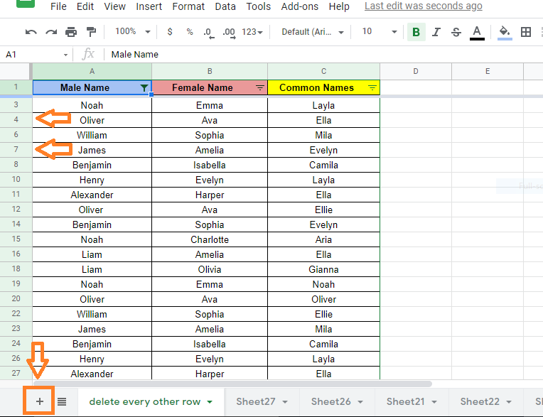
- Step 1: Select the columns where you want to delete the Nth row.
- Step 2: Now apply the filter to the selected columns using the Filter icon.
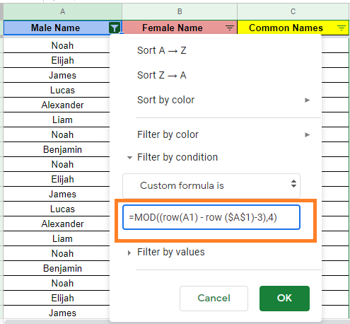
- Step 3: Once the filter is applied, click on the Filter icon in the column header.
- Step 4: Select Filter by condition and select “Custom Formula” from the drop-down menu.
- Step 5: Now enter the formula =MOD((row(A1) – row ($A$1)-3),4) in the empty field.
- Step 6: Press the “Enter” button and you will see the results.
Now copy-paste the results to another sheet in the spreadsheet to delete the hidden rows.
Explanation of MOD Formula in Google Sheets
MOD Function Syntax =MOD((row(A1) – row ($A$1)-{Nth -1}),{Nth})
- MOD(dividend, divisor): This is the modulus operator; we’re using it to hide or remove the cell if the division operation gives a remainder of “0.”
- Row: The value of a cell’s row is returned by ROW(cell reference). This is how we indicate that we’re looking at rows rather than individual cells.
- Offset: Determines which row begins the hiding/deleting period. Calculate the offset by subtracting 1 from your Nth factor to begin on the Nth cell after the header ( if N is 7, the offset is 6).
- The first row AFTER the header is hidden by -0.
- After the header, -1 starts obscuring the second row.
- After the header, -2 starts hiding the third row.
- After the header, -3 starts hiding the fourth row.
This pattern repeats itself until it shares the same value as N. After a certain point, you can’t use this formula to start hiding rows.
For example, if you want to delete every third row, use =MOD((row(A1) – row ($A$1)-2),3) and similarly for every tenth row, use the following formula =MOD((row(A1) – row ($A$1)-9),10.