Alternating Colors in Google Sheets: The Google Spreadsheets are adding new features from day to day to work efficiently. Sadly, we didn’t have the option to colour the alternate rows, so we had to rely on the Conditional Formatting function in Google Sheets to do so. However, the latest feature of Google Sheets allows us to color the rows alternatively. Within few clicks, we can color the rows alternatively in Google Sheets without any difficulty. On this page, let’s discuss how to select alternate rows in Google Sheets and color them.
Also, don’t miss out to check our article on important Google Sheets Tricks and Tips to work like a Pro in Google Sheets.
Color Alternate Rows in Google Sheets
Let’s consider we have the following dataset and now we would like to color the alternate rows.
- How to Extract the Year from Google Sheets-YEAR Function in Google Sheets
- How To Insert Indents in Google Sheets? – Know How to Tab Down in Google Sheets
- How to Make an Organization Chart in Google Sheets? – Create an Org Chart in Google Sheets
Follow the steps listed below to color alternative rows in Google Sheets:
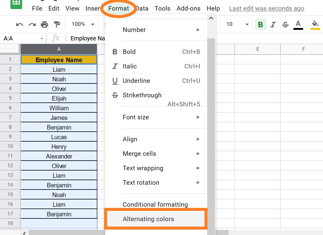
- Step 1: Select the cells where you would like to color the cells alternatively. (Make sure you are selecting headers as well.)
- Step 2: Click on the “Format” tab.
- Step 3: Select “Alternating Colors” from the drop-down menu.
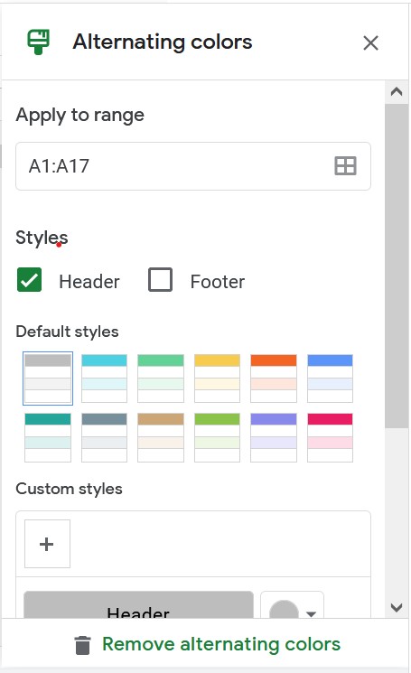
- Step 4: Now a new “Alternating Colors” Pane opens towards the right side of the screen.
- Step 5: In the Alternating Colors pane, select Headers under “Styles“.
- Step 6: You can select any of the default styles here from the list.
- Step 7: Alternatively, you can also custom your colors, headers and other cells under the “Custom Styles” window.
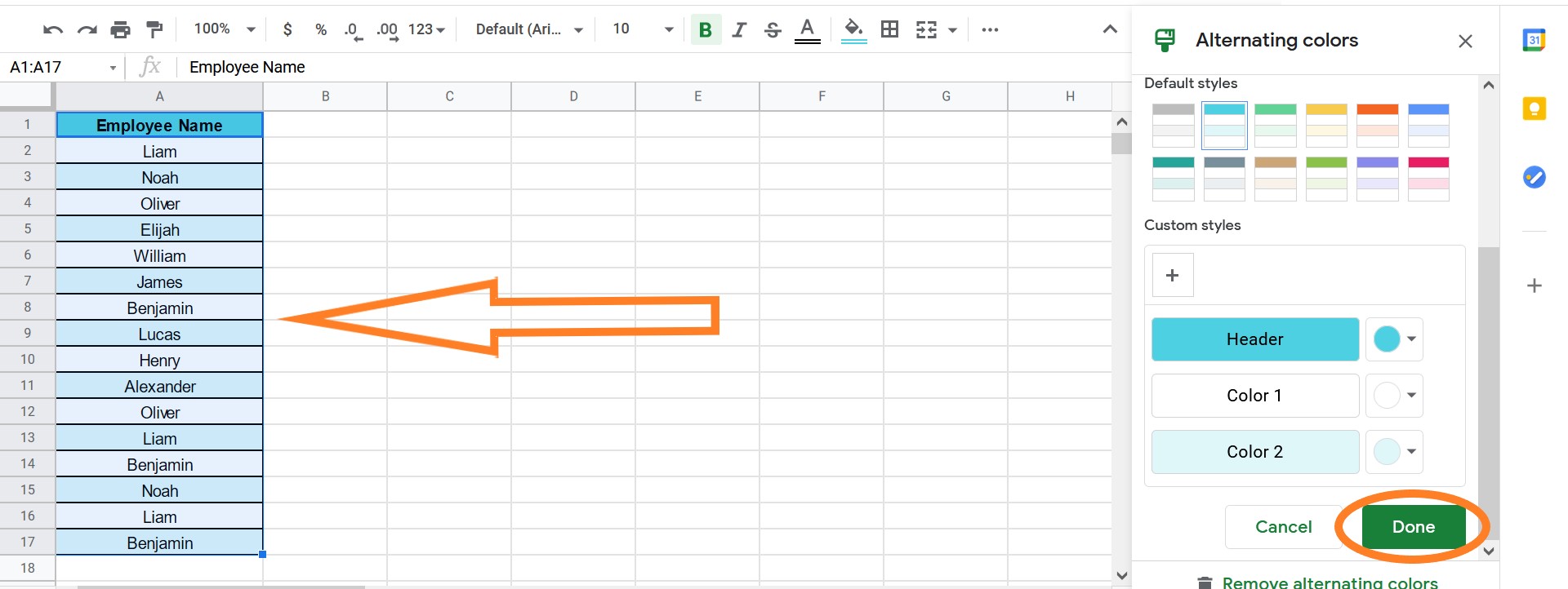
Now you will see the cells or the rows in Google Sheets coloured alternatively as shown below.
Color Alternate Rows in Google Sheets using Conditional Formatting
This method was used before the “Alternating Colors” feature was added to the Google Sheets. Follow the steps listed below to color the rows with alternative colors using the conditional formatting function.
- Step 1: Select the dataset, where you would like to color the cells alternatively.
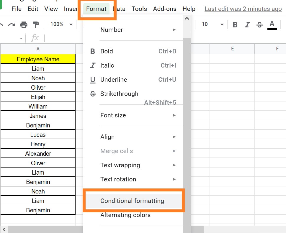
- Step 2: Click on the “Format” tab and select “Conditional Formatting“.
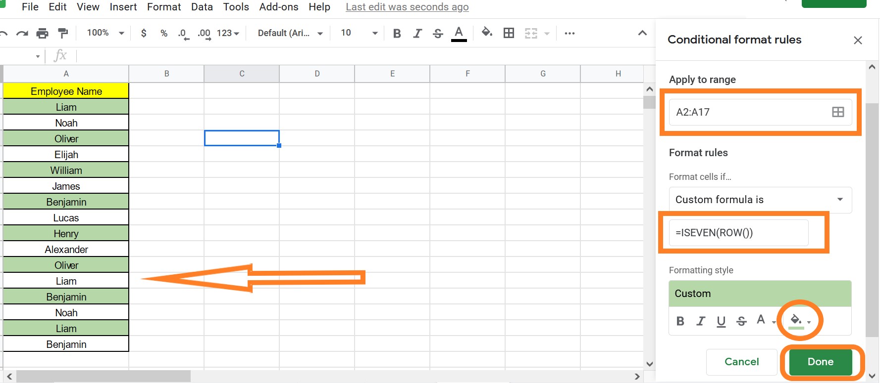
- Step 3: Now cross-check the Cell Range and select the “Add new rule“.
- Step 4: Under “Format Rules“, select the “Custom Formula is“.
- Step 5: Now type the formula as “=ISEVEN(ROW())“.
- Step 6: Under “Formatting Style” select the color under the “Fill Color” function.
- Step 7: Click on “Done“. You will see the results as given below.
Google Sheets Alternating Colors Every 2 Rows
If you want to color the rows every 2 rows or the third row, then you will have to use the “Conditional Formatting” function which is explained below.
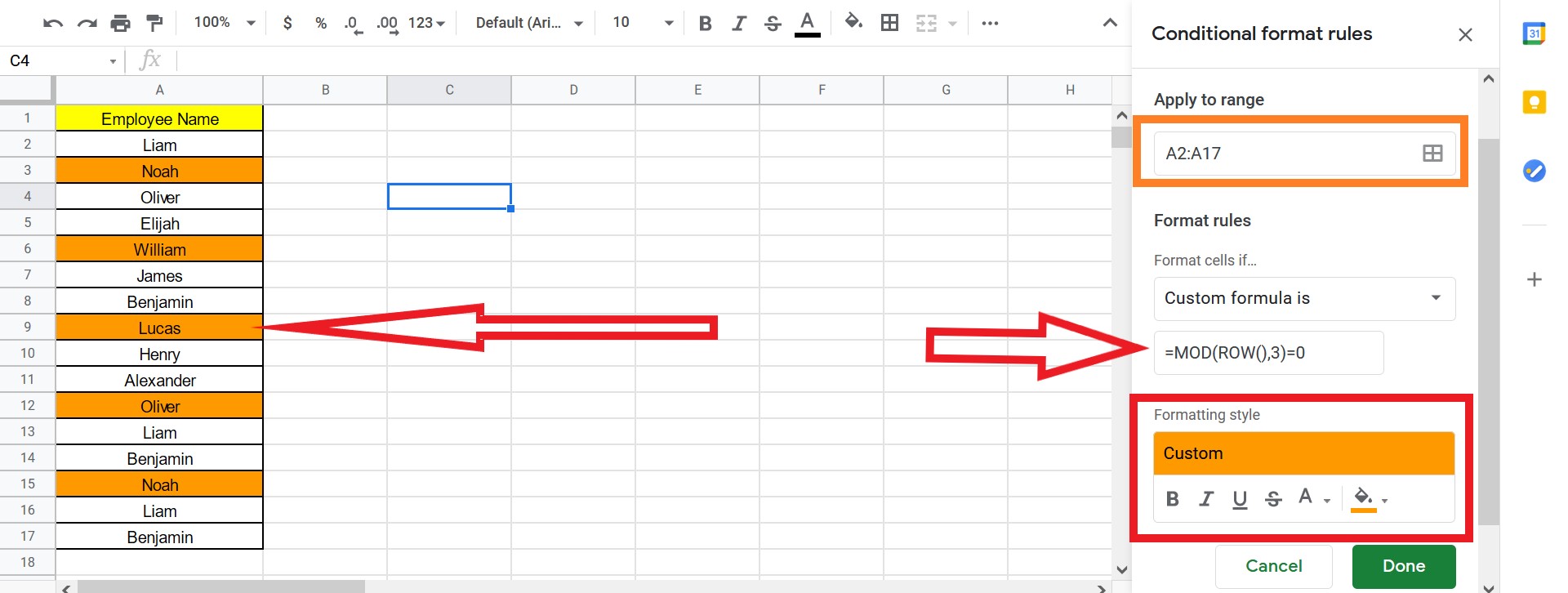
- Step 1: Choose the dataset where you’d like to color the third row or color after every 2 rows.
- Step 2: Select “Conditional Formatting” from the “Format” menu.
- Step 3: Select “Add new rule” and double-check the Cell Range.
- Step 4: Select “Custom Formula is” under “Format Rules.”
- Step 5: Now in the value or formula tab, enter the formula as “=MOD(ROW(),3)=0“
- Step 6: Select the colour from the “Fill Color” function under “Formatting Style.”
- Step 7: Hit the “Done” button. Now you will see the results.
Highlights of Alternating Colors in Google Sheets
- Google Sheets will automatically highlight the alternate rows in the colours you choose if you expand the dataset and add more records at the bottom.
- If you delete records, the colours will remain and you will have to remove them manually.
- Google Sheets will automatically update the colours if you add more rows to the dataset.
- If you already have a colour applied to the cells, it will be replaced by the colours you choose when using the ‘Alternating colors’ feature to highlight them.
- And when you remove the alternating colours, it will preserve the original colours while removing the alternate colours.
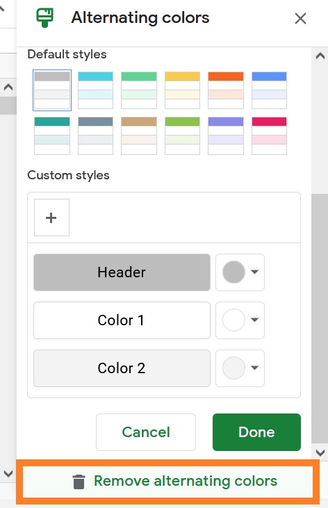
How To Remove Alternating Color in Google Sheets?
Select any cell in the dataset, go to the Format tab, and then to the ‘Alternating colors‘ option to remove the Alternating colour. This will bring up a window where you can ‘Remove alternate colors.’