The Ultimate Guide to Using Conditional Formatting in Google Sheets

Conditional Formatting in Google Sheets allows you to highlight cells that meet certain criteria. This can help you better understand spreadsheets at a glance and create spreadsheets that make them more human-readable. It’s also a great way to track goals, providing visual indicators of how you’re doing against specific metrics. In this article, let’s understand everything conditional formatting along with important Google Sheet tips. Read on to find out more.

Table of Contents How to Access Conditional Formatting in Google Sheets? Create Heatmap Using Conditional Formatting Highlight All Instances of Duplicate Data Points Conditional Formatting Cells Based on Another Cell Value Color Alternate Rows using Conditional Formatting in Google Sheets

How to Access Conditional Formatting in Google Sheets?

We can create n number of magics in Google Sheets using the conditional formatting function. Let’s understand how to access the Google sheets Conditional formatting with the help of the steps given below:

• Step 1: Select the Google Spreadsheet where you would like to use conditional formatting.
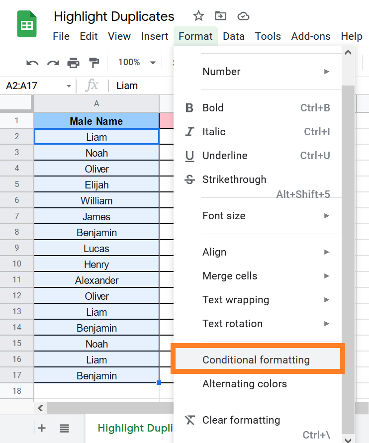
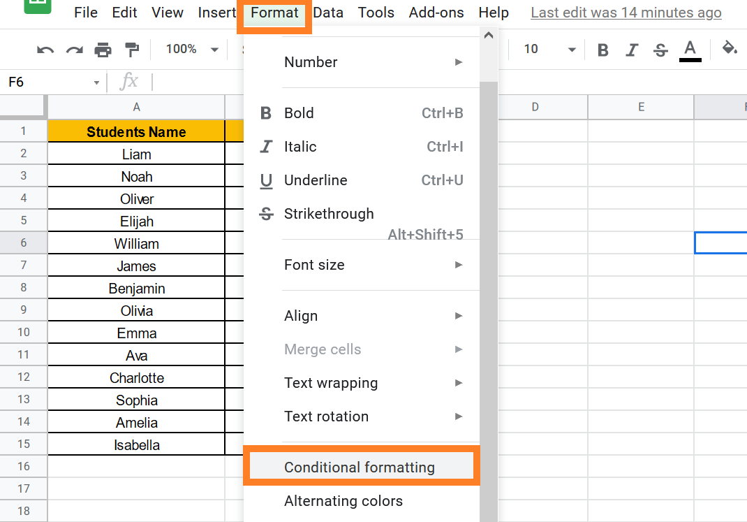
• Step 2: Choose the “Format” tab from the menubar.
• Step 3: Now a drop-down opens. Select “Conditional Formatting” from the drop-down menu.

• Step 4: A conditional formatting pane opens towards the right side of the screen as shown below.

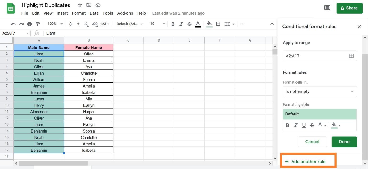
With the help of the Conditional Formatting pane, you can customize your Google Sheets.

• How to Insert Checkbox in Google Sheets: Add/Remove/Customize Checkbox
• How to Color Alternate Rows in Google Sheets: Alternating Colors Every 2 Rows, 3 Rows
• Conditional Formatting Based on Another Cell Value in Google Sheets

This brings up the ‘Conditional format rules’ pane on the right, where you can configure the rules. When you use conditional formatting in Google Sheets, you now have two options:

• Single Color: When you want to highlight all the cells based on their value, you can use the ‘single color’ option.
• Color Scale: When you want to visually present the difference between the values in the cells, you can use the ‘Color scale’ option.

Create Heatmap Using Conditional Formatting

Follow the steps listed below to create a heatmap using conditional formatting:

• Step 1: Choose the data set for which you want to generate the heat map.
• Step 2: Select Conditional formatting from the Format menu.
• Step 3: Select ‘Color scale’ in the Conditional formatting rules pane.
• Step 4: Cross-check the ‘Apply to range‘ option which refers to the correct range of cells. If not, you can change the range of cells from here.
• Step 5: Select the gradient you want from the Preview drop-down menu. It is important to note that the color on the left of the gradient is applied to the lower value numbers, while the color on the right is applied to the higher value numbers.
• Step 6: You can see a live preview in the data set while selecting the gradient here. In this case, we are using the red to green gradient.
• Step 7: Click the Done button.This will generate a heat map with a gradient-based on the cell value.

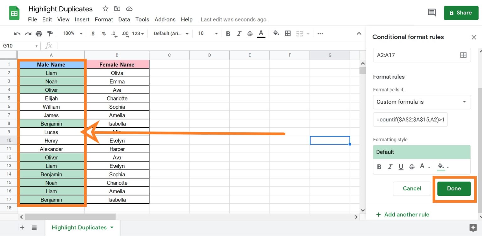
Highlight All Instances of Duplicate Data Points

In Google Sheets, you can use the custom function feature in conditional formatting to highlight duplicate data points.

Follow the steps below to highlight all instances of duplicate occurrence:

• Step 1: Choose a data set where you would like to highlight duplicate data points.
• Step 2: Select Conditional formatting from the Format menu.

• Step 3: Select ‘Single Color‘ in the Conditional Format rules.
• Step 4: Check that the ‘Apply to range‘ sections. If the cell range is selected wrongly, then correct cell range here.
• Step 5: Select the ‘Custom formula is‘ option from the ‘Format cells if‘ drop-down menu.
• Step 6: Fill in the following formula: =COUNTIF($A$2:$A$15,A1)>1

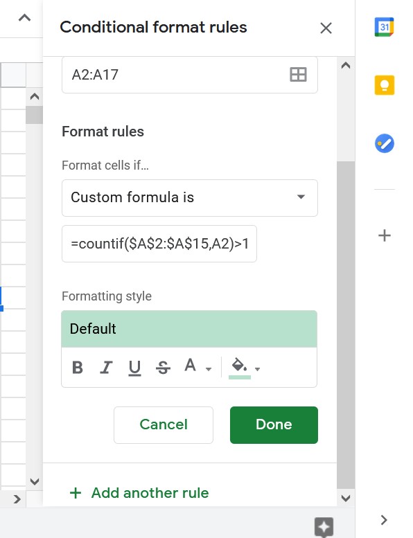
• Step 7: Choose a format.
• Step 8: Click the Done button.

When there are duplicate values, this will highlight all of them.

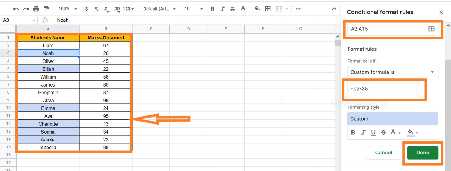
Conditional Formatting Cells Based on Another Cell Value

In Google Sheets, we may utilize conditional formatting based on another cell value to highlight names based on the student’s grade. Follow the steps given below to apply the conditions:

• Step 1: Select the cells you want to highlight.
• Step 2: Select “Format” from the drop-down menu.
• Step 3: From the drop-down option, choose “Conditional Formatting.” On the right side of the screen, a Conditional formatting pane will appear.

• Step 4: Now, as indicated in the figure below, pick “Single Color.”
• Step 5: From the drop-down menu, pick “Custom Formula” from the “Format Rules” section.
• Step 6: Write the formula as “=B2>35” in the Formula settings. (For the purposes of this discussion, we’ll use the number 35.)
• Step 7: Select the formatting options you want to use under the Formatting style option. We’ve decided on the color blue.
• Step 8: Click on the “Done” button. You will see the results.

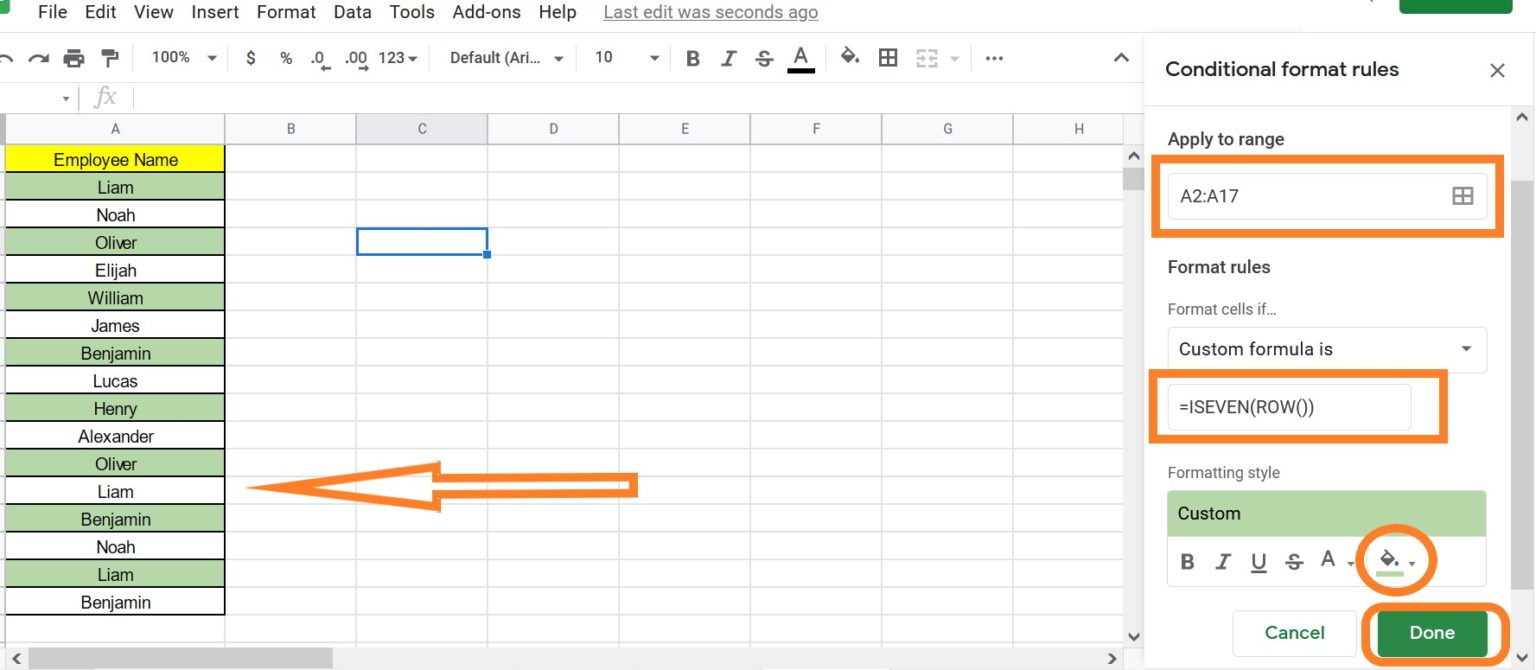
Color Alternate Rows using Conditional Formatting in Google Sheets

To use the conditional formatting feature to color the rows with alternate colors, follow the procedures mentioned below.

• Step 1: Choose the dataset where you’d like to alternately color the cells.
• Step 2: Select “Conditional Formatting” from the “Format” menu.
• Step 3: Next, double-check the Cell Range and click “Add new rule.“
• Step 4: Select “Custom Formula is” under “Format Rules.”
• Step 5: Update “=ISEVEN(ROW())” in the formula section.
• Step 6: Select the color from the “Fill Color” function under “Formatting Style.“
• Step 7: Select “Done” from the drop-down menu. You’ll see the results as shown below.