When working with Google Sheets, it’s no surprise to perform different operations with the dataset such as removing the last character from the string, trim the text, and so on. And if you are having a dataset where you would like to remove the last character or last 5, 4, 2, etc., characters from a string, then this article is for you. In this article, let’s understand how to remove the last character from a string with the help of Google Sheet tips provided on this page. Read on to find more.
Table of Contents |
How to Remove the Last Character of String?
We can remove the last character of the string with the help of the following 3 Google functions:
- LEFT Function =LEFT(A2, LEN(A2)-1)
- MID Function =MID(A2,1,LEN(A2)-1)
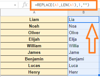
- REPLACE Function =REPLACE(A2,LEN(A2),1,””)
Now let’s understand how to remove the last characters of text in Google Sheets using the above functions with examples.
- How to Extract the Year from Google Sheets-YEAR Function in Google Sheets
- How to use REGEXEXTRACT Function in Google Sheets?(With Examples)
- REPT Function In Google Sheets – How To Repeat Rows in Google Sheets?
Using LEFT Function to Remove the Last Character from String
You can define the number of characters you want to extract from a string in a cell using the LEFT function in Google Sheets.
So, if you can figure out how many characters are in a cell, you can use the LEFT function to retrieve all of them except the last one.
Consider the following dataset where you would like to remove the last character from the string.
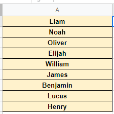
Now follow the steps listed below to remove the last character from the string using the LEFT function:
- Step 1: Open the Google Sheet where you would like to remove the last character from the string.
- Step 2: Now move the next cell to enter the LEFT function formula.
- Step 3: Type the formula as “=LEFT(A2, LEN(A2)-1)“.
- Step 4: Press the “Enter” button.
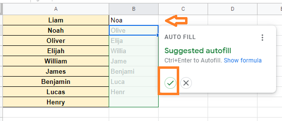
You will see the results.
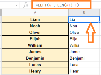
How to Remove the Last 3 Characters in Google Sheets?
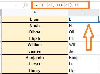
We can remove the last 3 characters in Google Sheets using LEFT Function. Just follow the steps listed in the above section and replace the LEFT formula as =LEFT(A2, LEN(A2)-3)
| No of Characters to be Removed | Formulas to be Used |
| To Remove the Last Character | =LEFT(A2, LEN(A2)-1) |
| To Remove the Last 2 Character | =LEFT(A2, LEN(A2)-2) |
| To Remove the Last 3 Character | =LEFT(A2, LEN(A2)-3) |
| To Remove the Last 4 Character | =LEFT(A2, LEN(A2)-4) |
| To Remove the Last 5 Character | =LEFT(A2, LEN(A2)-5) |
Using MID Function to Remove the Last Character from String
With the help of the MID function, we can easily remove the last character from a string. Follow the steps listed below to remove the last characters using the MID function in Google Sheets.
- Step 1: Open the Google Sheets where you would like to use the MID function.
- Step 2: Now move the adjacent cell.
- Step 3: Here type the MID formula as “=MID(A2,1,LEN(A2)-1)“.
- Step 4: Press the “Enter” button.
- Step 5: You will see the results. Now the drag the fill handle. By doing so, the MID formula will be applied to all the cells.
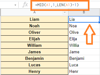
While the LEFT function extracts a defined number of characters from the left side of a string, the MID function extracts a specified number of characters from the middle.
Using REPLACE Function to Remove the Last Character of the String
Using the REPLACE function is another simple method to accomplish this. You can use the REPLACE function to replace the last character in a string with a blank character (which is equivalent to removing it).
Follow the steps listed below to remove the last character of the text using the REMOVE function:
- Step 1: Launch the Google Spreadsheet where you like to use REPLACE function.
- Step 2: Now move to the adjacent cell where you would like to remove the last character of the string.
- Step 3: Here enter the formula as =REPLACE(A2,LEN(A2),1,””) and Press the “Enter” button.
- Step 4: Now drag the fill handle from the formula applied cell to apply the same formula to other cells. You will see the results.
