Google Sheet conditional formatting functions analyze the value entered inside the cell and formats the cell according to specific conditions. In most cases, the current cell value is used to apply the conditional formatting there, but it can also be used to implement conditional formatting based on another cell value.
For example, let’s consider we have a bunch of students whose scoreboard is prepared using Google Sheets. Now we have to separate the students who have secured below 35 and the students who have scored more than 80 marks. In such cases, we can use conditional formatting on one cell with the name in another cell based on the student’s marks. Also at the end of the article, we have provided few Google Sheets tips on conditional formatting. Read more to find out.
Highlight Cells Based On Another Cell Value
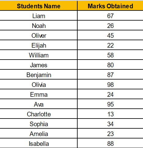
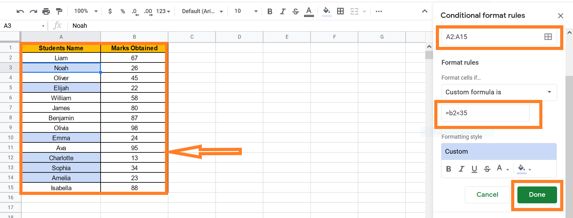
As discussed above, let’s take student scores as an example and see how students’ names can be highlighted based on their scores. Suppose you have the following data set and would like to highlight names that have a score of less than 35.
How Do You Conditional Format Cells Based On Another Cell Value?
We can use conditional formatting in Google sheets based on another cell value to highlight names based on the student’s score. To apply the conditions, follow the steps as listed below:
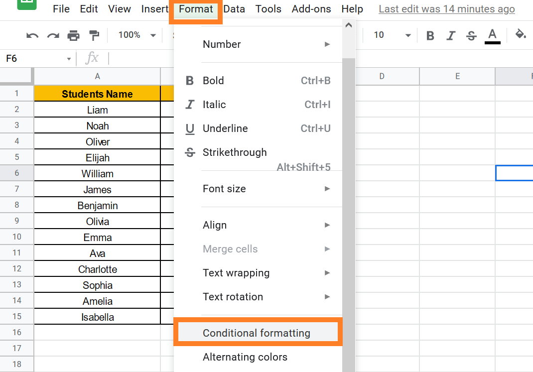
- Step 1: Choose the cells you wish to highlight. We are highlighting students names here
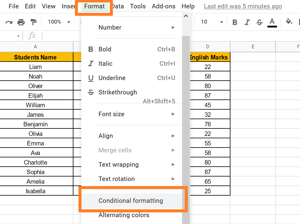
- Step 2: Click on the “Format” option.
- Step 3: Now select “Conditional Formatting” from the drop-down menu. Now a Conditional formatting pane will open towards the right side of the screen.
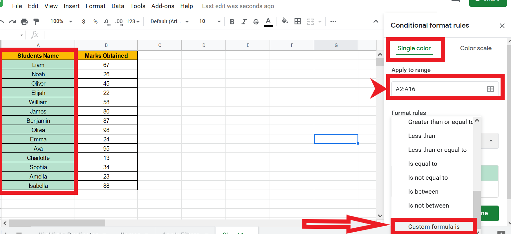
- Step 4: Now select the “Single Color” as shown in the image below.
- Step 5: Now click on the “Format Rules” and select “Custom Formula” from the drop-down menu.
- Step 6: In the Formula files, enter the formula as “=B2<35“. (We are considering 35 as the number here.)
- Step 7: Under the Formatting style option, select the formatting options which you would like to apply. Here we are choosing the Blue colour.
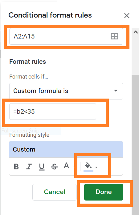
- Step 8: Now, click on “Done“. You will see the results.
How Does Conditional Format Cells Based On Another Cell Value Works?
Here we have chosen the cells with names and thus the cells with names are highlighted. Now to determine whether the selected formatting is to be applied to a cell or not, the condition specified simply must be checked. If TRUE is returned for the cell, the formatting will be used, otherwise, the condition will not.
- How To Highlight Duplicates In Google Sheets?
- How to Create a Grid Chart in Google Sheets? – Add Grid Lines and Borders in G-Sheets
- How to Create and Use Heat Map in Google Sheets With Examples
Here we have used the formula = B2<35 for each cell. Therefore, if conditional formatting is the cell A2, the condition is checked to B2<=35, and when cell A3 is checked, this condition is checked to B3<=35 and so on.
Since the value of B3 is 26, the cell returns True and highlights the cell in blue colour as per our colour specifications.
Highlight Cells Based On Another Cell Value In Multiple Cells on Google Sheets
In the above example how to highlight a value-based cell in another cell. The same logic can be extended and the values in multiple cells can be used to highlight a cell on Google Sheets.
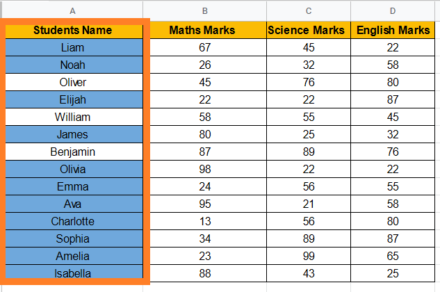
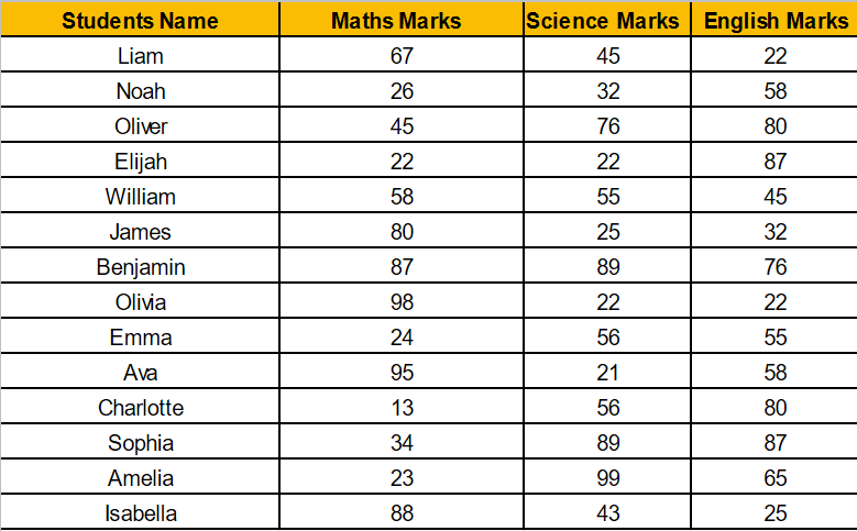
For example, consider the data set below and now we should highlight all student names in each of the three topics, whose score is less than 35. For this to work, three different cell values should be analysed and the name of the student should be highlighted if any cell value (score) is less than 35.
Follow the steps listed below to highlight cells using Conditional Formatting based on multiple other cell values in Google Sheets.
- Step 1: Select the cells which you would like to highlight. (Here we are highlighting the students’ names.)
- Step 2: Now click on the “Format” tab and select “Conditional Formatting” from the drop-down menu.
- Step 3: Now “Conditional Formatting Pane” will open on the screen. Make sure, you are under the “Single Color” tab as shown in the image below.
- Step 4: Click on the “Format Rules” and select the “Custom Formula is“.
- Step 5: Now in the “Value or Formula” field, enter the formula as “=OR(B2<35, C2<35, D2<35)“
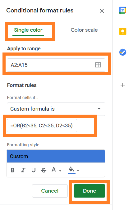
- Step 6: Move to the “Formatting Style” window and select the formatting types such as colours which you would like to apply. Here we have chosen the “Blue” colour.
- Step 7: Click on “Done“.
The results will be displayed on selected cells as shown below.