Grid Charts are a special type of chart in Google Sheets that help us understand the data in a more easy-to-understand format. Grid Charts are usually used to represent datasets such as student grades, employee workforce, weather reports, and much more. However, there is no inbuilt feature with the help of which we can build grid charts in Google Sheets. But still, you can easily devise a grid chart in Google Sheets using the formulas and functions. This page will tell you everything about how to create a grid chart in a spreadsheet with the help of the Google Sheets Tips provided on this page. Read further to find out more.
| Table of Contents |
Google Sheets Grid Chart
Let us take an example from a student’s scorecard. We will create a grid chart that shows the performance of the students in their board exams. When creating a chart, we simply change the percentages in the cell that will automatically change the colours of the grid that we have devised in the spreadsheet.
- How to Make a Line Chart in Google Sheets: Setup/Edit/Customize Line Graph
- How to Make an Organization Chart in Google Sheets? – Create an Org Chart in Google Sheets
- How to Create a Gantt Chart in Google Sheets? (Dynamic Gantt Chart Formula)
How to Create a Grid Chart in Google Sheets?
Follow the steps which are outlined below to create a grid chart in Google Sheets.
- 1st Step: Launch Google Sheets on your device.
- 2nd Step: Move to the cell where you want to enter the percentage value. In this example, we have used cell A1 with a percentage value of 85%.
- 3rd Step: Now we have to create a 10 x 10 grid in Google Sheets. For this, move to the cell where you want to create a grid and enter the formula as =SEQUENCE (10,10). In this post, I am using Cell A3 to enter the sequence formula.
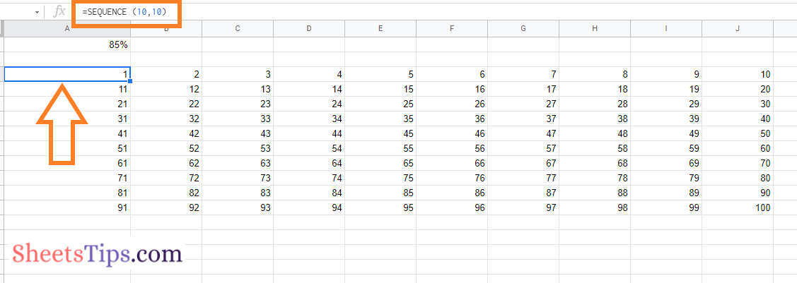
- 4th Step: This will result in 10 X 10 grids in ascending numbers from 1 to 100.
- 5th Step: The next step is to adjust the columns and row sizes. Using the fill handle, adjust the column height and width to make it square.
- 6th Step: Wrap the sequence function with an IF statement and an ArrayFormula to determine whether the value in a particular cell is greater than the threshold percentage. As a result, our formula will be =ArrayFormula(IF (SEQUENCE (10,10) > A1*100,2,1).
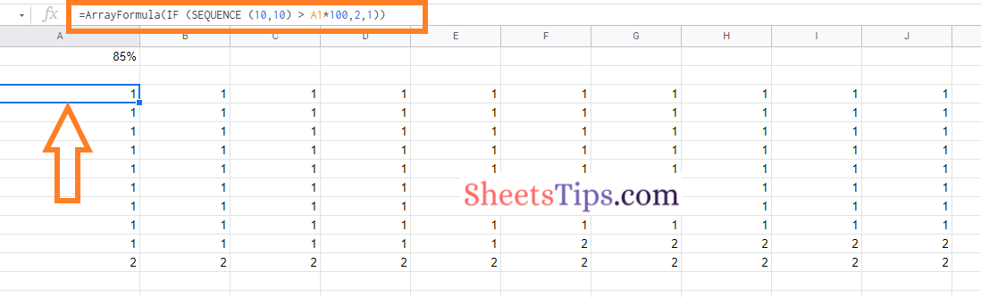
- 7th Step: Press the “Return” key and you will see the results as shown in the image above.
Customising the Grid Chart in Google Sheets
- 1st Step: Select the sequence range.
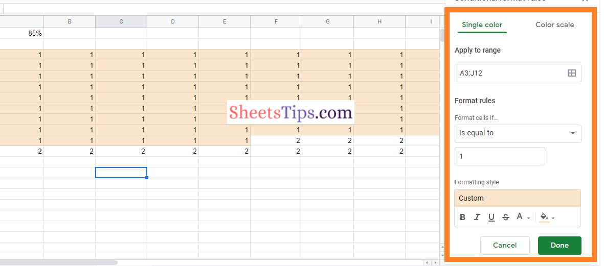
- 2nd Step: Choose “Format” and select “Conditional Formatting” from the drop-down menu.
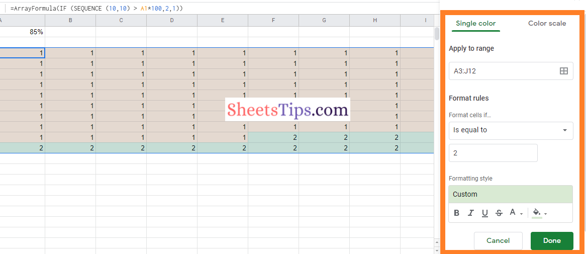
- 3rd Step: In the Format Rules drop-down section, choose “is equal to” and enter 1 in the value or formula section.
- 4th Step: Now the next step is to move to the “Formatting Style” and choose the “Color” as per your requirements.
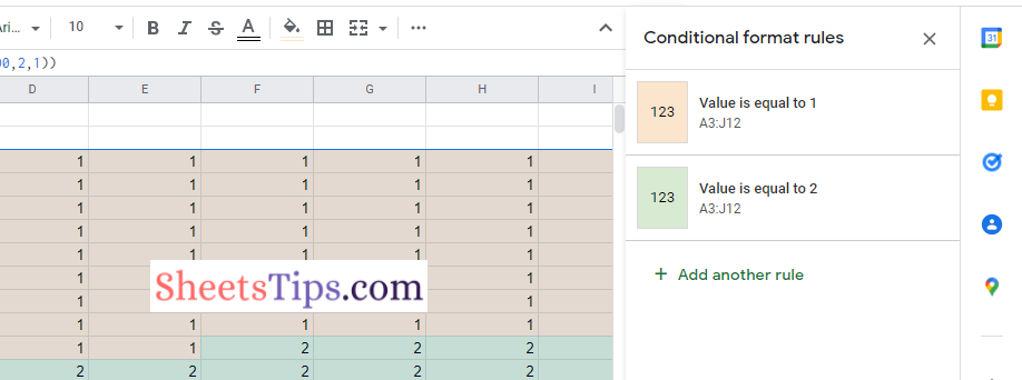
- 5th Step: Apply the second conditional formatting to the same sequence and enter the number as 2 instead of 1.
- Now you will see the colour is added to your grid chart.
- 6th Step: Now select the grid that was created by you and then choose “Format” > “Number” > “More Formats” and “Custom Number Format“.
- 7th Step: Here the “Custom Number Format” section will open on the screen. In this section, paste this emoji: “
 “.
“.
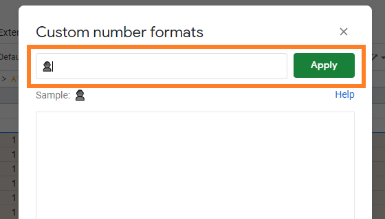
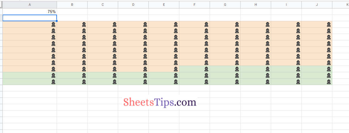
- 8th Step: This converts all values to emoji, regardless of whether they are 1 or 2. Finally, align the values horizontally and vertically by centering them.
- 9th Step: That’s it. When you change the percentage value, the chart will automatically adjust as shown below.