A Gantt chart is a type of bar chart that is widely used to show how a project’s schedule is broken down into tasks or events and plotted against time. With the help of this Chart, one can easily understand the flow of the projects and so on.
However, Google Sheets doesn’t have default chart options with the help of which we can create Gantt Charts. To overcome this issue, we can easily create a Gantt Chart using the Dynamic Gantt Chart Formula. So even if you are looking at how to create a Gantt Chart, then this page will explain everything about it. Let us learn everything about Gantt Chart using the Google Sheets Tips provided on this page. Read further to find more.

Table of Contents |
Pre-Requisites to Create Gantt Chart in Google Sheets
- In order to create a Gantt Chart first, we will have to create a dataset. For this launch Google Sheets on your devices
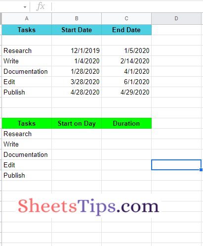
- In this article, we are using an example that talks about the project of publishing an article. Now we have to create a dataset which talks about the project cycle of publishing an article. To get this done, first, we will have to create a dataset with three columns namely – Tasks, Start Date, End Date, and fill in all the necessary details.
- Then, off to the side or beneath the previous table, create a similar table that will be used to generate the graphs in each section of the Gantt chart. To create the Gantt chart, the table will contain three headings: tasks, start day, and task length. Here don’t fill in any of the details and keep all the cells empty.
Refer to the following image and create a dataset that is similar to your Google Sheets.
- How To Sync Charts From Google Sheets to Google Docs & Google Slides?
- How to Make an Organization Chart in Google Sheets? – Create an Org Chart in Google Sheets
- How to Make Dot Plot in Google Sheets? Customizing Scatter Chart to Dot Plot
Steps to Create Gantt Chart in Google Sheets
The steps to create a Gantt Chart in the Google Spreadsheet are explained below:
- 1st Step: Open the Google Spreadsheet on your device that has the dataset which is similar to that of the above image.
- 2nd Step: Now on the homepage, move to the second data set which is unfilled. These cells will be filled out using Google Sheet Gantt Chart Formula.
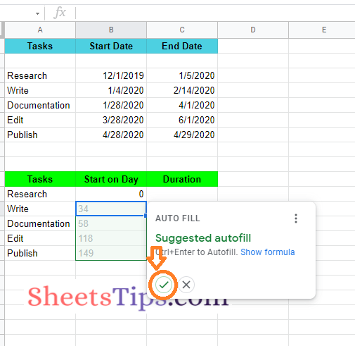
- 3rd Step: In cell B11, enter the formula “=INT(B3)–INT($B$3)” and press the “Enter” button.
- 4th Step: If the Formula auto fill is suggested use the same else drag the formula applied cells to other cells to apply the same formula.
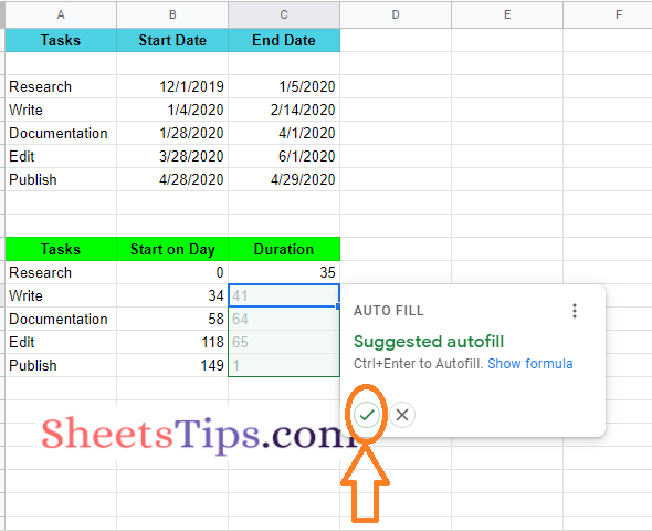
- 5th Step: Then move to column C11 and enter the formula as “=(INT(C3)–INT($B$3))–(INT(B3)–INT($B$3))” and press the “Enter” button.
- 6th Step: If the AUTO FILL is suggested, click on the Tick (✓) mark. Else drag the formula applied cell drop down to the other parts of the cell to apply the same formula.
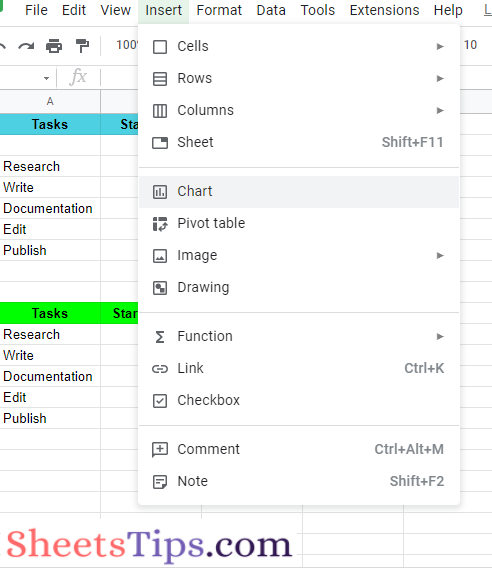
- 7th Step: Now select the second dataset and click on the “Insert” tab.
- 8th Step: Choose “Chart” from the drop down menu.
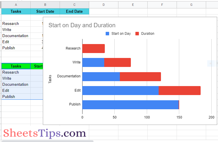
- 9th Step: Here based on the dataset, the Google Sheet will automatically insert a Chart. Luckily, Google Sheets here inserted a Stacked Bar Chart.
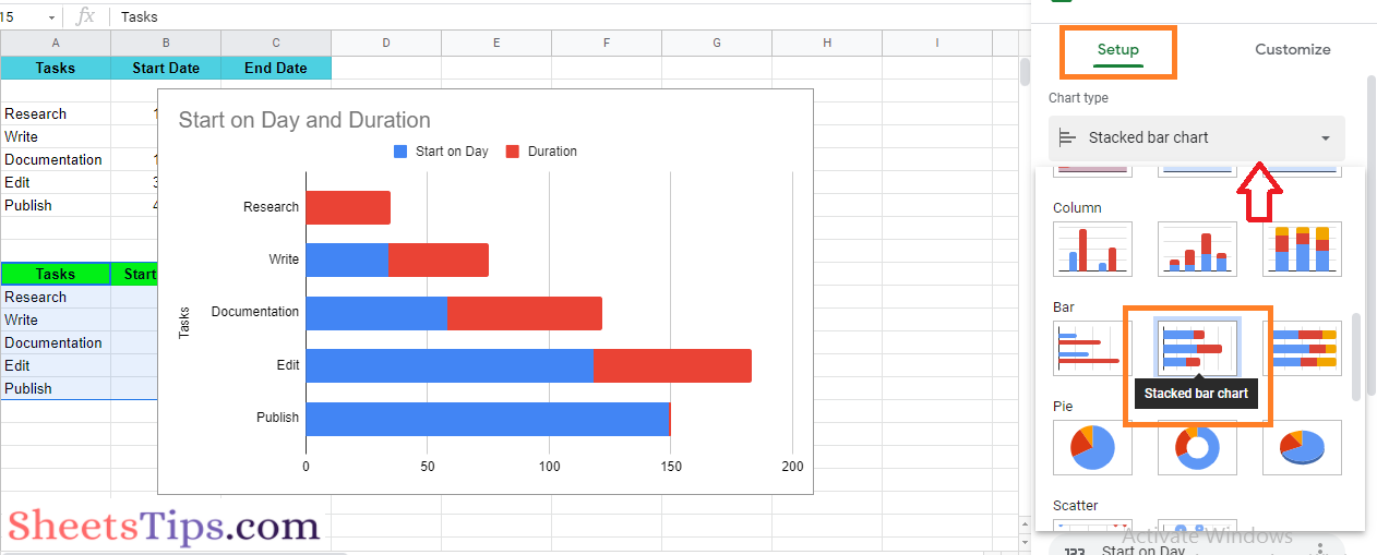
- 10th Step: If Google Sheets hasn’t inserted a Stacked Bar Chart, then move to the Chart Editor Pane and choose the “Setup” section.
- 11th Step: Move to the Chart Type section and scroll towards down and choose “Stacked Bar Chart” under Bar Chart Types as shown in the image below.
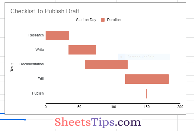
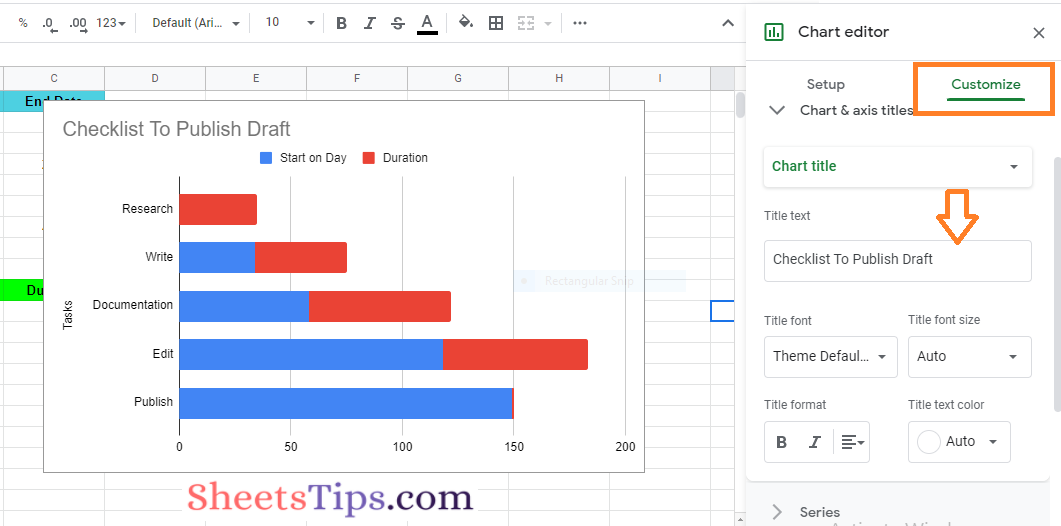
- 12th Step: Now move to the “Customize” section and edit the Chart title as per your requirement. Here we are creating a title text as “Checklist To Publish Draft” as shown in the image below.
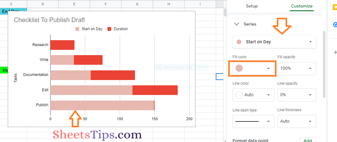
- 13th Step: Now move to the series section, and choose the first series Fill Color as per your requirements. In our example, we are changing the Blue color to Peach color as shown in the image below.
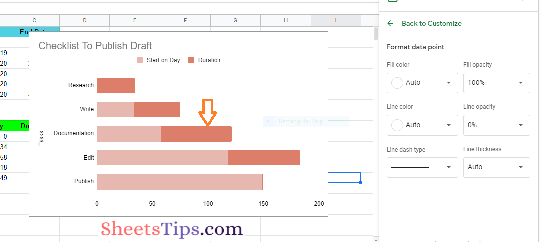
- 14th Step: Now change the second series color as per your requirements by following the same method as per the 13th step.
- 15th Step: Now edit the start on day series fill color into white color to transform it as Gannt Chart as shown in the image below.
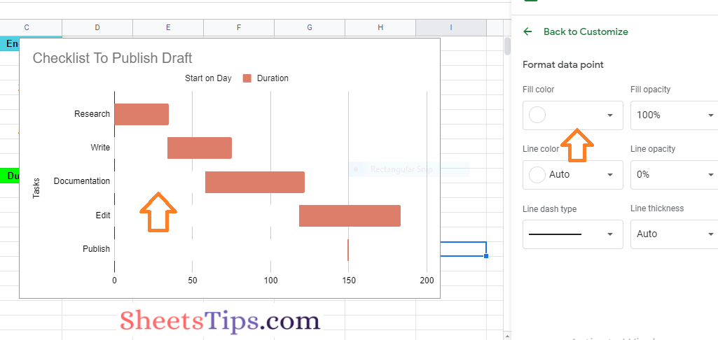
That’s it, the Gannt Chart has been created on the Google Sheets using the Stacked Bar Chart as shown in the image below.