
It’s no wonder that Google Sheets allows users to perform various operations using the functions and formulas available on Google Sheets. Similarly, in this article, let us consider an example where we want to construct a single-cell formula that accepts a string of search terms and returns all of the results that have at least one phrase in the Terms column that matches. Sounds difficult? Don’t worry. Using the Google Sheets Tips and Tricks provided on this page, let us understand how to build this complex formula in the spreadsheet. Read further to find out more.
| Table of Contents |
How to Match Words in Google Sheets?
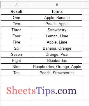
Before getting into the details of how to match the words in Google Sheets, let us first create a dataset. In our dataset, in Column A, let us have the “Result” phrases that should be matched with terms. In Column B, we will have to create the terms to which the results need to be matched. So our dataset will be like the following image.
- How to Use INDEX MATCH Functions in Google Sheets with Google Sheets
- How To VLOOKUP In Google Sheets Using Wildcards For Partial Matches?
- How to Convert Rows to Columns or Backwards in Google Sheets?
Google Sheets Search for Text in Range – Steps
Now follow the steps as listed below to filter out the matching keywords in the Google Spreadsheet.
- 1st Step: Open the Google Sheets on your device that has the dataset.
- 2nd Step: Now, move to the column where you want to search and get the matching results. In this example, I am using Columns E and F as an example.
- 3rd Step: In Column E, enter the search term. In this example, I am using the search term “raspberries, orange, apple.“
- 4th Step: In column F, enter the formula, which will result in the matching terms in cell E2. So our formula here will be “=FILTER
". - 5th Step: Enter the above formula and press the “Return” key and now you will see the results as shown in the image below.
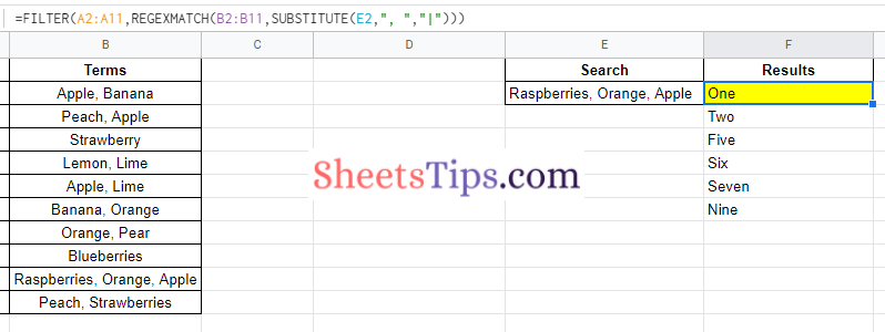 From the above image, we can see that the terms are matched to the results.
Formula Explanation: The SPLIT function separates the three fruits in cell E2 into separate cells. Then, using the pipe “|” delimiter, we join them back together.
Alternative Formulas for Matching Terms in Google Sheets
Alternatively, you can replace the existing formula with the following formulas to get the same results:
- =FILTER(A2:A11,REGEXMATCH(B2:B11,JOIN(“|”,SPLIT(E2,”, “))))
- =QUERY(A2:B11,”select A where B contains ‘”&JOIN(“‘ or B contains ‘”,SPLIT(E2,”, “))&”‘”)