
Wildcards are an extremely versatile collection of symbols that allow you to choose a group of comparable strings at the same time. Google Sheets allows us to use the Wildcards with the VLookup function to find a value or symbol that is not an exact match but the partial match.
For example let us say, you want to extract all the URLs with the name amazon. You can do this manually when your dataset is small, however, if your dataset is huge, then you can simply use the VLookup function with Wildcards to extract all the URLs having the term amazon.
On this page, let us understand how to use the VLookup wildcards in Google Sheets with the help of Google Sheets Tips. Read further to find more.
Table of Contents |
VLOOKUP Wildcard Google Sheets
The list of wildcards that we can use along with the VLOOKUP function is as follows:
- The asterisk (*): When we use the asterisk as a wildcard, it finds all the matches related to it. For example, if you use the asterisk to find the word Ama, then it will match all the partial matches such as amaz, amazon, amazons, and so on.
- The Question Mark(?): A question mark is used to represent a single character. For example, if you use “a?a”, then the possible results would be ama, aha, aia, aba and so on.
- The tilde(~): This wildcard generally comes before one of the above wildcard characters (* or?) and tells Google Sheets that the next character should be treated as a regular character symbol rather than a wildcard. For instance, the string (~) indicates that we wish to find all strings that include the identical text t.
How To Use VLOOKUP Wildcard Partial Match in Google Sheets?
So here is a list of URLs from various websites.

- How to Use Wildcards in Google Sheets with Examples?
- How to Analyze Data from Google Sheets with Examples
- How to Use the INDEX function in Google Sheets (Examples)
Now we need to find the value in the source table which is a partial match but not the exact match. Let us say that we need to extract the URL with the name Amazon. Here in the table, there is no string with the name amazon as an actual match, but with the help of the VLOOKUP wildcard, we can extract the partial match. The steps to get this done in Google Sheets are as follows:
- 1st Step: Open the Google Spreadsheet on your device and move to the dataset where you want to perform the partial match with the help of Google Sheets VLookup Wildcards.
- 2nd Step: Now on the homepage, move to the cell where you would like to extract the results.
- 3rd Step: Simply enter the formula =VLOOKUP(“*”&C2&”*”,$A$2:$A$6,1,FALSE) – {modify the formula as per your datarange}
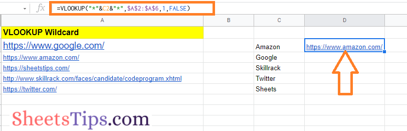
- 4th Step: Now press the Return key and you will see the result.
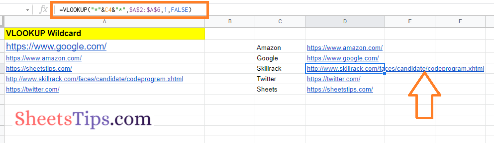
- 5th Step: Simply drag the fill handle and you will see the partial matches being loaded as shown in the image below.
Google Sheets VLookup Wildcard in Table Array Formula Explanation
Rather than utilizing the standard VLOOKUP formula “=VLOOKUP(C2,$A$2:$A$6,1,FALSE)”, We used wildcards by placing an asterisk on both sides of the cell reference C2, as seen below.
=VLOOKUP(“*”&C2&”*”,$A$2:$A$6,1,FALSE)
This ensured that the VLOOKUP function searched the source table for any text that contained the term in cell C2, regardless of whether it was preceded or followed by certain letters.
As a result, the formula will seek a match, and if one is found, it will provide the whole URL for the given term.