Every Google Spreadsheet user will have to learn how to use the Wildcard characters. Generally, in Google Sheets, we can combine wildcard characters with functions to perform a variety of useful opeartions. In this article, let us explore how to use wildcards with the help of Google Sheet tips provided on this page.
Table of Contents |
What is Wildcard in Google Sheets?
When you use a wildcard symbol, you can represent any character by using that symbol instead of the actual characters themself. For specific results, they are often used in combination with other query functions like conditional functions, search and lookup functions, and filtering.
In Google Sheets, there are three wildcard characters and they are:
- Asterisk (*): Any character or any number of characters is represented by an asterisk (*).
- Question Mark (?): One character is represented by the question mark wildcard (?).
- Tilde (~): You can also use the Tilde (~) to tell Google Sheets not to use any wildcard characters (such as * and ? ). Google Sheets will know if you search for “m~?” and not use the question mark as a wildcard in this case if you use “m?” as an example in your search.
How to Use Wildcards Using SUMIF Function? (* Wildcard)
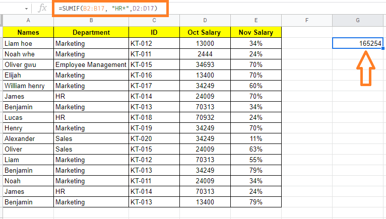
Let us consider the following dataset. Here we want to calculate the October salary of HR department employees.
Now follow the steps listed below to use Wildcards using SUMIF Function in Google Sheets:
- Step 1: Move to the cell where we want to get the results. In our case, we are using cell G2.
- Step 2: Now type the formula as “=SUMIF(B2:B17, “HR*”,D2:D17)“.
- Step 3: Press the “Enter” button.
Now you will see the results as shown below.
- How To VLOOKUP In Google Sheets Using Wildcards For Partial Matches?
- Remove Last Character from a String in Google Sheets (or Last N Characters)
- Comparison Operators in Google Sheets (>,<,<>,=,>=,<=)
Formula Explanation:
In the above example, we have used the condition “HR*” which means find all the cells which contain the word HR. Now the spreadsheet will not search for the exact match, but it searches all the cells which contain the word “HR” along with other characters.
Once similar texts are found, the SUMIF function will calculate the total salary value
When a match is found, the SUMIF function adds the October salary value corresponding to the matching cell to the list of Total Salary values that have been selected. The SUMIF function sums up the selected Total salary values and displays the result in cell G2 once it has finished going through all of the models.
In other words, the wildcard ‘*’ aided in the discovering of various variations of the search term ‘HR’ in column B.
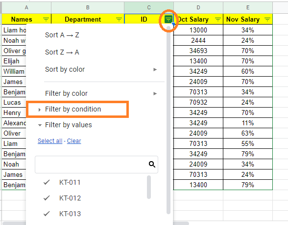
Using Wildcards to Filter Data Based on Conditions in Google Sheets (? Wildcard)
Wildcards can also be used to quickly and easily filter data based on a condition. Let us start with the same dataset as shown in the image below:
Assume you want to filter the data so that only cells beginning with the letter K and ending with the number 2 are visible. This is very easy to execute by using the question mark wildcard with the help of the steps given below:
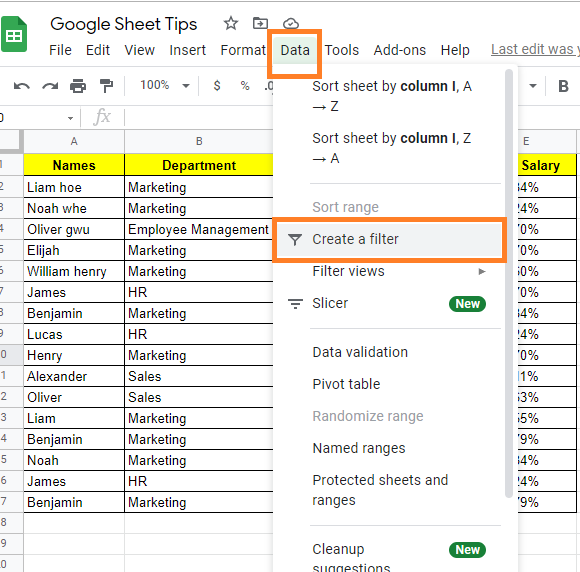
- Step 1: Select the range of cells that you would like to filter.
- Step 2: Click on the “Data” menu from the toolbar and choose “Create a Filter” from the drop-down menu.
- Step 3: Now click on the “Filter” icon against the “ID” column.
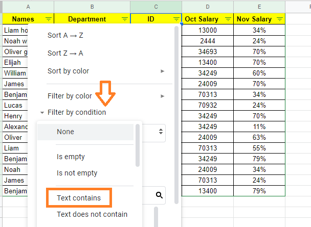
- Step 4: A sub-menu will open up on the screen. Select the “Filter by Condition” option.
- Step 5: Now choose “Text Contains” from the drop-down menu.
- Step 6: Here a new input box will appear on the screen. Here you will have to enter the formula.
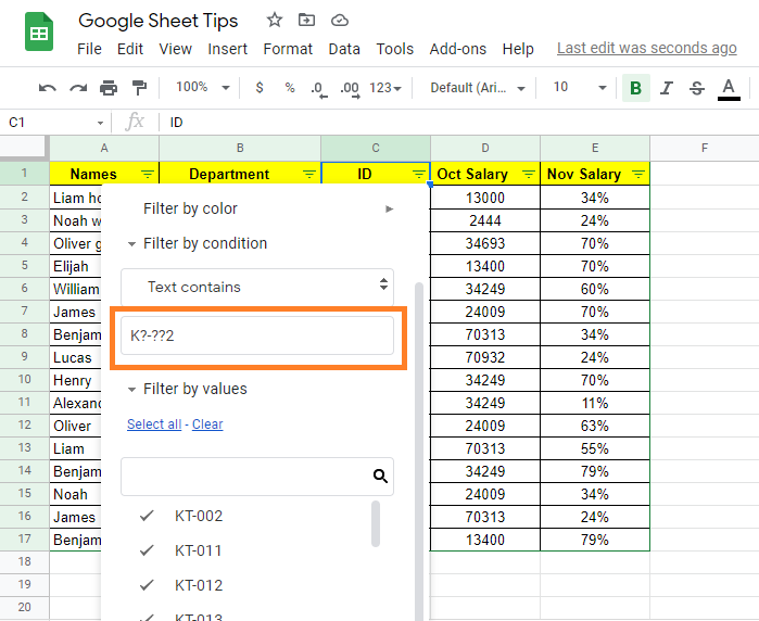
- Step 7: Type the search string or formula as ‘K?-??2‘.
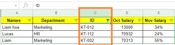
- Step 8: Click on the “Ok” button and you will see the results.
How to Use Wildcards Using COUNTIF Function? (Tilde ~)
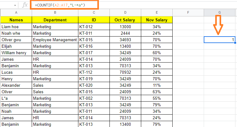
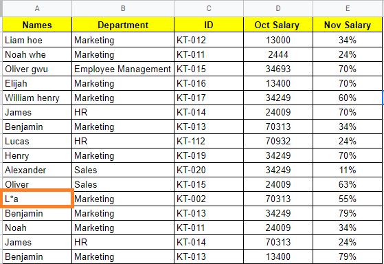
Although the tilde wildcard (~) isn’t used very often, it’s still useful to know how to utilize it. Let us understand how to use the Tilde ~ wildcard using the COUNTIF function. Consider the following dataset. Here we need to find out the string which exactly has the word “L*a”.
Let us understand how to achieve the same with the help of the steps given below:
- Step 1: Move to the cell where you would like to extract the string which has the word “L*a”.
- Step 2: Now enter the formula using the COUNTIF function as “=COUNTIF(A2:A17,“L~*a”)“
- Step 3: Press the “Enter” button. Now you will see the results as shown below.