
In Google Sheets, the INDEX function is used to extract data from a cell or a range of cells. By passing a specific range, a row, and a column to the function, we may specify which cell or range of cells we wish to extract. The INDEX function returns the cell or array of cells at the intersection of the supplied range’s row and column. In this article, let us understand how to use the INDEX function with the help of Google Sheet tips provided on this page. Read on to find more.
Table of Contents |
Syntax of INDEX Function in Google Sheets
The Google Sheets INDEX function using reference are given below:
INDEX(reference, [row], [column])
This syntax makes use of the cell reference form of input. Here,
- reference: In order to extract data from a set of cells, we need a reference range.
- row: row is the row number in the table (within the reference range) from which we wish to get the data.
- column: column denotes the desired data extraction column within the database. This parameter can be deleted.
The above syntax will return the value of the cell whose row and column indexes intersect at the intersection supplied in the reference parameter.
- Google Sheets QUERY Function Explained With Examples
- How to VLOOKUP from Another Sheet in Google Sheets: Vlookup Between Two Sheets
- How to Use Filter Functions in Google Sheets with Examples
The Google Sheets INDEX function using an array is given below:
INDEX(array, row, [column])
This syntax takes advantage of the array input form.
- array refers to a set of cells or a set of array constants from which we want to extract data.
- row is the array row from which we wish to get the data. If the column parameter is given, then this is not required.
- column is the array column that contains the data we wish to retrieve. If the row parameter is given, this is not required.
How to use the INDEX Function in Google Sheets?
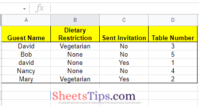
To know how to use the INDEX function in Google Sheets, let us consider the following dataset. This dataset contains a guest list along with invitation details to an event.
Using INDEX and Match Function to Return Cell Value
In the above dataset, I want to check the Dietary Restriction of Mary. To know the same using the INDEX formula, follow the steps as listed below:
- Step 1: Move to the row where you would like to extract the Dietary Restriction of Mary.
- Step 2: Now enter the formula “=INDEX(A1:D6, MATCH(“Mary”, A1:A6, 0), 2)“.
- Step 3: Press the “Enter” button and you will see the results.
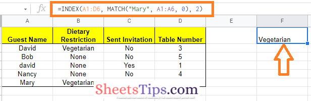
Here the row number is dynamic and the column number is hardcoded.
Using INDEX Function with Array to Extract a Row of Data
You can use the INDEX function to retrieve the values from multiple cells in a row or column at once. INDEX returns an array formula including all four 3rd row values, so you will need it.
To get the data from all four cells in the 3rd row, follow the steps as listed below:
- Step 1: Select the row where you need to extract the results.
- Step 2: Make sure you have enough empty cells where you want to extract the results.
- Step 3: Now type the formula as “=ArrayFormula(INDEX (A2:D7,3,0))”.
- Step 4: Press the “Enter” button.
Now you will see the results as shown below.
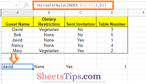
Because you used 3 as the row number and 0 as the column number, the formula works. In this case, you will obtain an array containing all the data from row 3 because row 3 is the one that pertains to “David”.
Using INDEX Function with Array to Extract a Column of Data
You may also get the values from all the cells in a certain column in your data set. To get the names of all the guests, follow the steps as listed below:
- Step 1: Move to the cell where you would like to extract the guest names in the column manner.
- Step 2: Make sure you have enough empty columns where you are trying to extract the data.
- Step 3: Now enter the formula as “=ArrayFormula (INDEX(A2:D7,0,1))“.
- Step 4: Press the “Enter” button and you will see the results as shown below.
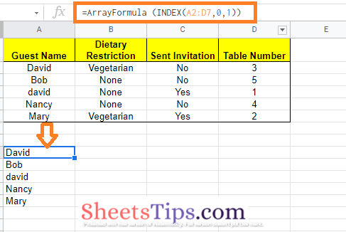
Formula Explanation: Because you entered 0 as the row number and 1 as the column number, the calculation works. Because the ‘Guest Name‘ column is the first one in the selected range, you will get an array with everything in column 1.