
Google Sheets comes with various functions such as VLOOKUP, IMPORTRANGE, REGXREPALCE, and so on. The FILTER function is one such amazingly strong one where we can perform various options without using the FILTER Views.
On this page, let’s learn everything about Filter Functions and operations that can be performed with the help of Google Sheet tips provided on this page. Read on to find more.
Syntax for Using Filter Functions in Google Sheets
The syntax for Filter Functions in Google Sheets are given below:
FILTER(range, condition1, [condition2, …])
- range – the filtered data should be within this range.
- condition 1: The condition on which the data is filtered is condition 1.
- condition2: additional conditions that the data is filtered based on.
It’s important to remember that the FILTER function only returns data that meets all of the specified criteria.
Highlights of Filter Functions in Google Sheets
- The FILTER function returns an array as a result. This means you won’t be able to remove a portion of the result.
- Filter Functions will produce a #N/A error if there is no match based on the conditions you gave.
- The formula will return a REF error if any cell that is expected to be filled by the result of the FILTER function is already filled.
Now that we are aware of the syntax of FILTER functions in Google Sheets. In the below section, let us understand how to use Filter Functions with examples.
- How to Create Filter Views in Google Sheets? (Share/Delete/Save/Duplicate Filter Views)
- How to Use OR Function in Google Sheets With Examples (Logical Functions)
- Google Sheets QUERY Function Explained With Examples
Filter Functions using Single Condition in Google Sheets
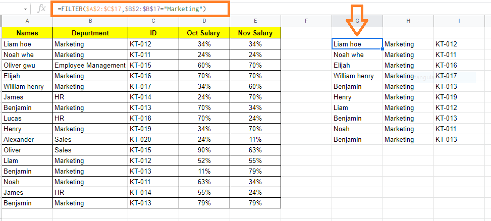
Let us consider we have an employee dataset and we need to filter only the employee who are belonging to the marketing department. Now follow the steps listed below to achieve the same:
- Step 1: Move to the cell where you would like to use the Filter Functions.
- Step 2: Now enter the formula using Filter function syntax. In our case, we are using the formula as “=FILTER($A$2:$C$17,$B$2:$B$17=”Marketing”)“.
- Step 3: Press the Enter button. Now you will see the data being filtered out without using inbuilt filter options.
Filter Functions using Multiple Condition in Google Sheets
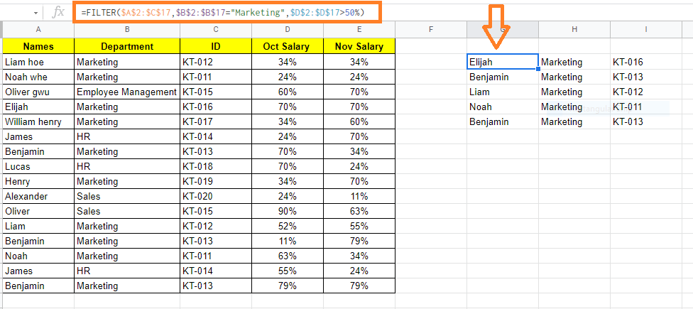
Let us say, in the same dataset, I want to extract the employee data who are working under the marketing department and along with it, I also want to extract whose salary was greater than 50%.
Now follow the steps listed below to achieve the same.
- Step 1: Move the cell where you want to extract the data using the filter function.
- Step 2: Now use the formula as “=FILTER($A$2:$C$17,$B$2:$B$17=”Marketing”, $D$2:$D$D17>50%)
- Step 3: Press the “Enter” button. The results will be as shown in the image below.
Filter Functions using Odd/Even Condition in Google Sheets
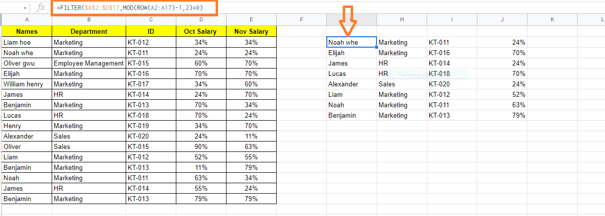
It’s really simple to extract all the even-numbered rows or the odd-numbered rows from a dataset using the FILTER function.
Let us consider the same dataset where we need to filter even rows and odd rows using Filter functions. To get this done, follow the steps listed below.
- Step 1: Move to the cell where you would like to use the Filter Function.
- Step 2: Now use the formula “=FILTER($A$2:$D$17, MOD(Row(A2:A17)-1,2)=0)”.
- Step 3: Press the “Enter” button. This will filter all the even-numbered rows as shown below.
Since we have represented row 1 as headers, Google Sheets ignores row 1 and starts counting from Row 2.
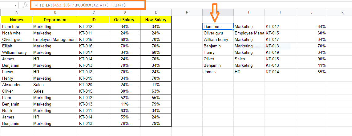
To filter the odd number of rows, use the formula =FILTER($A$2:$D$17, MOD(Row(A2:A17)-1,2)=1)
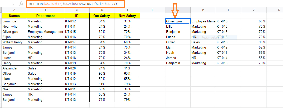
Filter Functions using ABOVE/BELOW Average in Google Sheets
You can apply conditions like the data points (or records) should be above or below average when using the FILTER function.
Let us understand how to use above or below Average functions in Google Sheets by following the steps listed below:
- Step 1: Move to the cell where you would like to use the AVERAGE Function in Google Sheets.
- Step 2: Now enter the formula as “=FILTER($A$2:$D$17,$D$2:$D$17>AVERAGE($C$2:$D$17)“.
- Step 3: Press the “Enter” button. You will see the results as shown below.
Here we have used the above Average function.
The formula to use the below-average function in Google Sheets is =FILTER($A$2:$D$17,$D$2:$D$17<AVERAGE($C$2:$D$17).
Also Read: Python Interview Questions on Data Types and Their in-built Functions