
Google Sheets Array Formula: An array, as we all know, is a collection of similar kinds of data in the form of rows and columns that helps in storing, arranging, and manipulating records. In Google Sheets too, we will need to encounter arrays along with various calculations based on their records, which might be tricky as well as time-consuming if you do not know the actual formulas.
This article will walk you through the basic formulas you will need to know when working with arrays in Google Sheets. Stay tuned till the end to unleash more of these important Google Sheet Tips.
- What is the Array Formula in Google Sheets?
- Google Sheets Array Formula Examples
- Matrix Calculations using Array Formula
- Use of COUTIF and SUMIF Array Formula Google Sheets
- Using Google Sheets Array Formula VlookUp
- What is the Google Sheets Array Formula to Ignore Blank cells?
- What is the Array Formula to Concatenate in Google Sheets?
- Fix Array Formula not Working Google Sheets
What Is the Array Formula in Google Sheets?
An array formula basically allows us to retrieve a range of cells as an output rather than a single value. We can also use non-array functions with arrays, like a range of data. To use array functions in Google Sheets, either type ARRAYFORMULA directly or press Ctrl+ Shift+ Enter (Windows) or Cmd+ Shift+ Enter (Mac) while keeping your cursor pointed to the formula bar.
This is one single formula that works for a huge data set. It is expandable which expands down the entire database if there is some change in a single place. Also, the Array Formula is dynamic. This means that if a new row is inserted, the formula will automatically be applied to it as well.
Syntax for ARRAY FORMULA: = ARRAYFORMULA( Array_Formula ), where, the parameters include:
- a cell range as reference.
- mathematical calculative expression using ranges having the same cell size.
- a function returning a value greater than one cell.
Google Sheets Array Formula Examples
Let’s visualize an array as a matrix that has a set of organized values in the form of rows and columns. Let’s consider the following table as an example. The set of values present within A1 to D3 is an array with 3 rows and 4 columns. The Array formula is applied to these elements of the array to perform multiple calculations and return a single value or a set of values in the form of a new array.
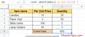
Let’s say we want to find the grand total of sales without creating an extra column. Follow these steps:
- Step 1: Click on the cell where you wish to display the result of the grand total of sales.
- Step 2: Next, enter the syntax =SUM( ARRAYFORMULA( B2: B5* C2: C5) ) and hit Enter.
Matrix Calculations using Array Formula
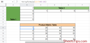
Well, did you know we can perform matrix multiplications using the Array formula as well? Let’s take an example to help us understand this better. Consider we have a row matrix called Table1 having 5 rows and a column matrix named Table2 having 4 columns.
- Step 1: To calculate the product of these two matrices, click on the cell where you wish to map the new result matrix and type the array formula: =ArrayFormula(C2:F2*B1:B5).
- Step 2: Press Enter and the result is going to be a 5×4 matrix that has the product of Table1 and Table2:
Use of COUTIF and SUMIF Array Formula Google Sheets
Array formulas can also be used with aggregation functions like SUMIF, SUMIFs, COUNTIF, and COUNTIFs, which help in quickly summing up values from a range after matching certain conditions.
Let’s take an item-wise sales table as an example here:
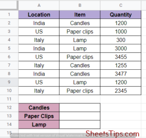
Our aim is to calculate the total sales with respect to each item and display the final results in cell locations F3:F5. If we use a SUMIF function here, we need to apply the formula thrice, i.e., once for each item, since the SUMIF function only satisfies one condition at a time. Using the Array Formula, we can specify a range of cells in the given condition as follows:
=ArrayFormula( SUMIF( B2:B10, A12:A14, C2:C10) )
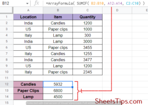
The second parameter says A12: A14 to help us achieve results for all three items at once! Since SUMIFs and COUNTIFs return the sum of an array after satisfying multiple criteria, the result only needs to be a single value. Hence, we can’t use them directly. Instead, if we use the ampersand operator (&) with our array formula, then we can expand our SUMIF function over the entire column.
The formula must be: =ArrayFormula( SUMIF( A2: A10& B2: B10, B12: B14& A12: A14, C2: C10) ), where:
- The item in column B must match the item in the corresponding cell in column E.
- The Outlet in column Column A must match with the outlet in column F.
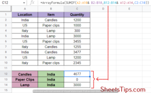
Here, we simply combined the range cells with their corresponding criteria by using the ampersand & operator first and then wrapped an Array Formula function along with the SUMIF formula. Now, the SUMIF function shows results based on more than one criteria.
Using Google Sheets Array Formula VlookUp
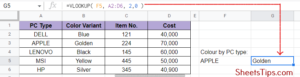
The VLOOKUP function is mainly used to sort an array and search for specific information based on a given condition. The syntax we need to follow here is: =VLOOKUP( search_key, cell_range, index, [ is sorted ] ).
Let’s take the following table, for example, where we see records on various computers based on their type, colour variant, cost, etc. Let’s say we want to extract the colour of the PC by putting its type as an input. For example, take the F5 cell, for example, to input the PC type and then go to the G5 cell and type the formula: =VLOOKUP( F5, A2: D6, 2,0 ). Now, type the PC type on F5 and get its colour displayed on the G5.
What Is the Google Sheets Array Formula To Ignore Blank Cells?
While entering data manually onto your Google Sheets, you may leave some spaces blank mistakenly.
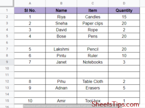
These blank spaces, if not paid attention to, may clash with the array formulas and result in incorrect outputs. Let’s see the steps to remove such blank rows:
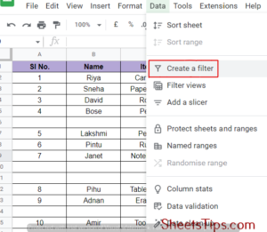
- Step 1: Select the entire table and then click on the Data menu, followed by Create a filter. This will create a filter for all the column heads.
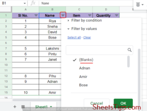
Step 2: Click on any one of the filters, select only (blanks) from the drop-down menu that appears, and click Ok. This will extract and display only the blank cells.
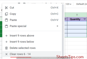
Step 3: Next, select all 4 rows and click on clear the rows from 6 to 15.
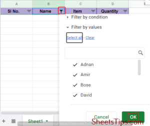
Step 4: Next, again click on one of the filters and click on Select All followed by the Ok button.
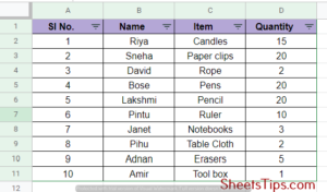
Your Array table is now ready with no blank cells.
What Is the Array Formula to Concatenate in Google Sheets?
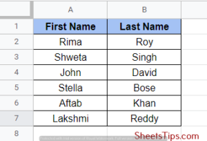
Concatenation in an array basically means combining the values of two arrays adjacently. We can use array formulas here to combine columns from multiple arrays and concatenate the values contained in them. Let’s take a table having a list of first and last names as an example.
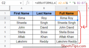
Our aim is to combine these two columns and concatenate their values to give us a new column named Full Name. Follow these steps:
- Step 1: Create a new column with the name Full name and click on the cell from where you wish to display the concatenated column.
- Step 2: Next, type the formula =ARRAYFORMULA( A2:A7& ” “& B2:B7) and press Enter.
The final result will be a new column with the first name and last name combined, along with a space in between. We can use the concatenation operator for numbers, dates, or any type of special character as well.
Fix Array Formula Not Working Google Sheets
Always make sure you are using the latest version of Google Sheets to work with. If you are using a version of Excel prior to 2019, the Ctrl+Shift+Enter method will not work to enter the Array Formula. Older versions of Google Sheets also do not support the aggregate and sum product functions. Also, if you see your spreadsheet is crashing, try to refresh your page by pressing the keyboard F5 key and starting again.
Recommended Reading On: Java Program to Print Zig-Zag Matrix Number Pattern