When we use the functions INDEX and MATCH separately we see that we have only limited options to perform operations. However, when both INDEX and MATCH are combined together, we can make most of it in Google Sheets.
On this page, we will look at how to utilize the INDEX and MATCH functions together, as well as some examples, with the help of Google Sheet tips. Read on to find out more.
Table of Contents |

MATCH Function in Google Sheets
Google Sheets MATCH function returns an item’s relative position in a range that matches a given value. The syntax of the MATCH function in Google Sheets are given below:
=MATCH(search_key, range, [search_type])
- search key – The value to look for in the search.
- range – The search range is a one-dimensional array. MATCH function will return #N/A! if the height and width of the range are both greater than 1.
- search type [ OPTIONAL – 1 by default ]- The method for doing a search.
- 1 – MATCH assumes the range is sorted in ascending order and returns the greatest value less than or equal to the search key when set to 1.
- 0 – In cases where the range is not sorted, a value of 0 indicates an exact match, which is necessary.
- -1 MATCH assumes the range is ordered in descending order and returns the smallest value greater than or equal to the search key if -1 is specified.
INDEX Function in Google Sheets
Google Sheets INDEX function accepts a cell range, a row index, and a column index, and returns the value in the cell that is at the intersection of the row and column specified. The syntax of the INDEX function is:
INDEX(reference, [row], [column])
- Reference: The range of cells from which we want to extract the item is referred to as reference.
- Row: The row offset from which we wish to extract the item is row inside reference.
- Column: column is the reference column offset from which we wish to extract the item. This parameter is not required.
How to Combine INDEX and MATCH Functions in Google Sheets?
When the two formulas are combined, they can search up a value in a table cell and return the same value in another cell in the same row or column. The general method to combine both INDEX and MATCH functions in Google Sheets are given below:
=INDEX(range2,MATCH(search_key,range1,0))
- range 1: The value we want to look for in range1 is the search key.
- search_key: The MATCH function determines the index for a value that matches the search key from a range of cells called range1.
- range2: The INDEX function extracts a value corresponding to the position/index returned by MATCH from the range2 of cells.
In other words, the MATCH function supports the INDEX function in determining the value to return’s location.
- How to Use the INDEX function in Google Sheets (Examples)
- How to VLOOKUP from Another Sheet in Google Sheets: Vlookup Between Two Sheets
- How to Use SWITCH function in Google Sheets? (With Examples)
Now that we understood the syntax and formula combination of INDEX and MATCH functions. In the next section, let us understand how both the function work together with examples.
Using INDEX and MATCH Function with Single Criteria References
Consider the following employee dataset. In the following dataset, we have employee name, ID, department, salary details. Now in the same dataset, towards the right side, we can see the employee Name and department box.
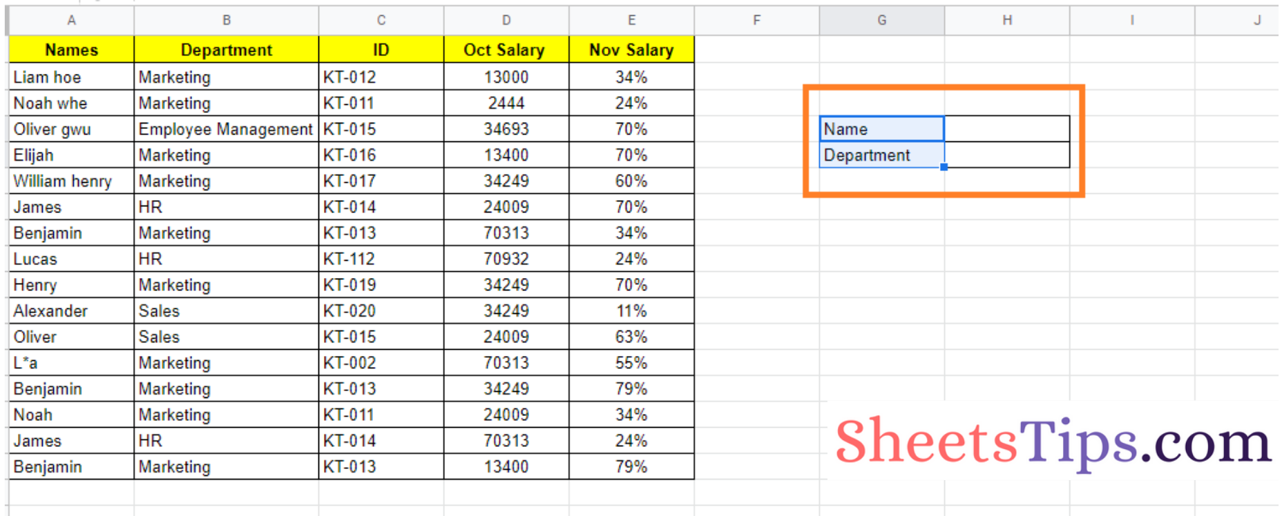
Now, if we want to change the employee departments’ names based on the employee name, we can combine both INDEX and MATCH functions in Google Sheets.
The steps to achieve the same are listed below:
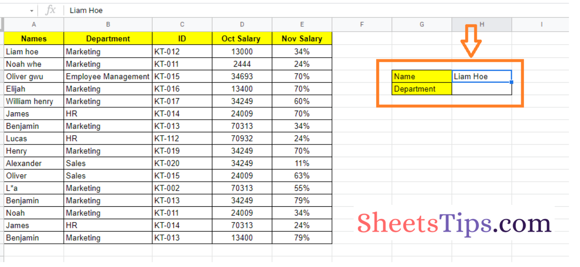
- Step 1: Move to the cell which is against the employee name cell and type the employee name whose department you would like to find.
- Step 2: Then move the cell against the department name.
- Step 3: Now enter the formula =INDEX(B2:B17,MATCH(H4,A2:A17,0))
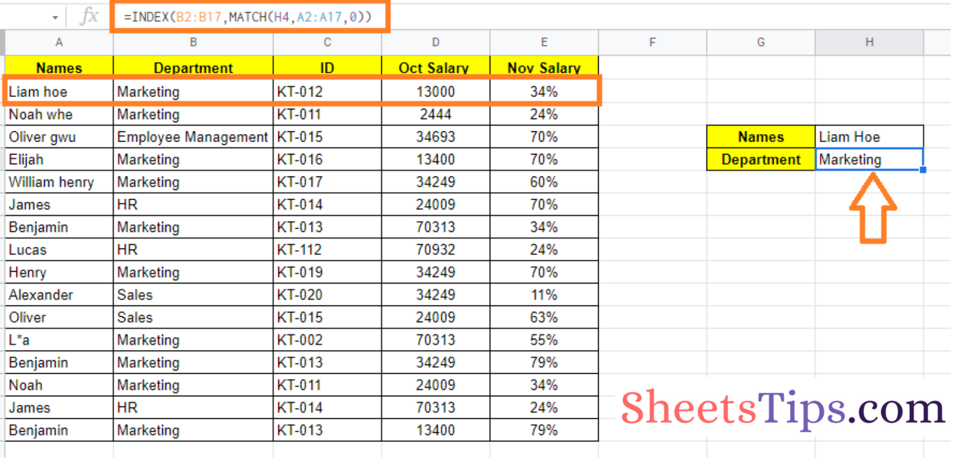
- Step 4: Press the “Enter” button. You will see the results as shown below. Now try to change the employee name and you will see department name changing as well.
Formula Explanation:
Let’s break down this formula to see how it worked. We’ll start with the formula’s inner function:
MATCH(H4,A2:A17,0)
This function searches the range A2:A17 for the value H4 and returns its position in the range.
Let’s have a look at the formula’s outer function next:
=INDEX(B2:B17,MATCH(H4,A2:A17,0))
This formula searches the range B2:B17 for the value in the 4th slot and returns that value, which is ‘Marketing.’
Using INDEX and MATCH Function with Multiple Criteria References
The range in the preceding example was a single column. The INDEX-MATCH operations, on the other hand, can give us additional versatility by allowing us to access a value from many columns.
Let’s assume that in cell G6 of our example worksheet, we can have either Department name, Salary, or even ID as a label. What if, in addition to the label in cell G6, the label in cell G6 was dynamic and subject to change?
In that instance, we would have to think about many columns, and the column we would go to would be determined by the label in cell G6. Well, this can be achieved by following the steps as listed below:
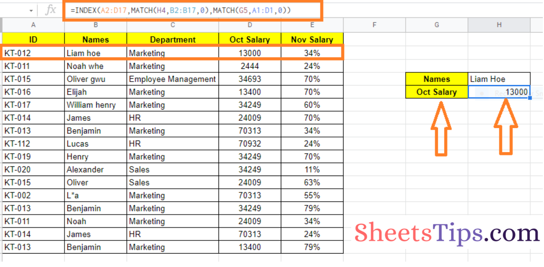
- Step 1: Move to the cell against the salary.
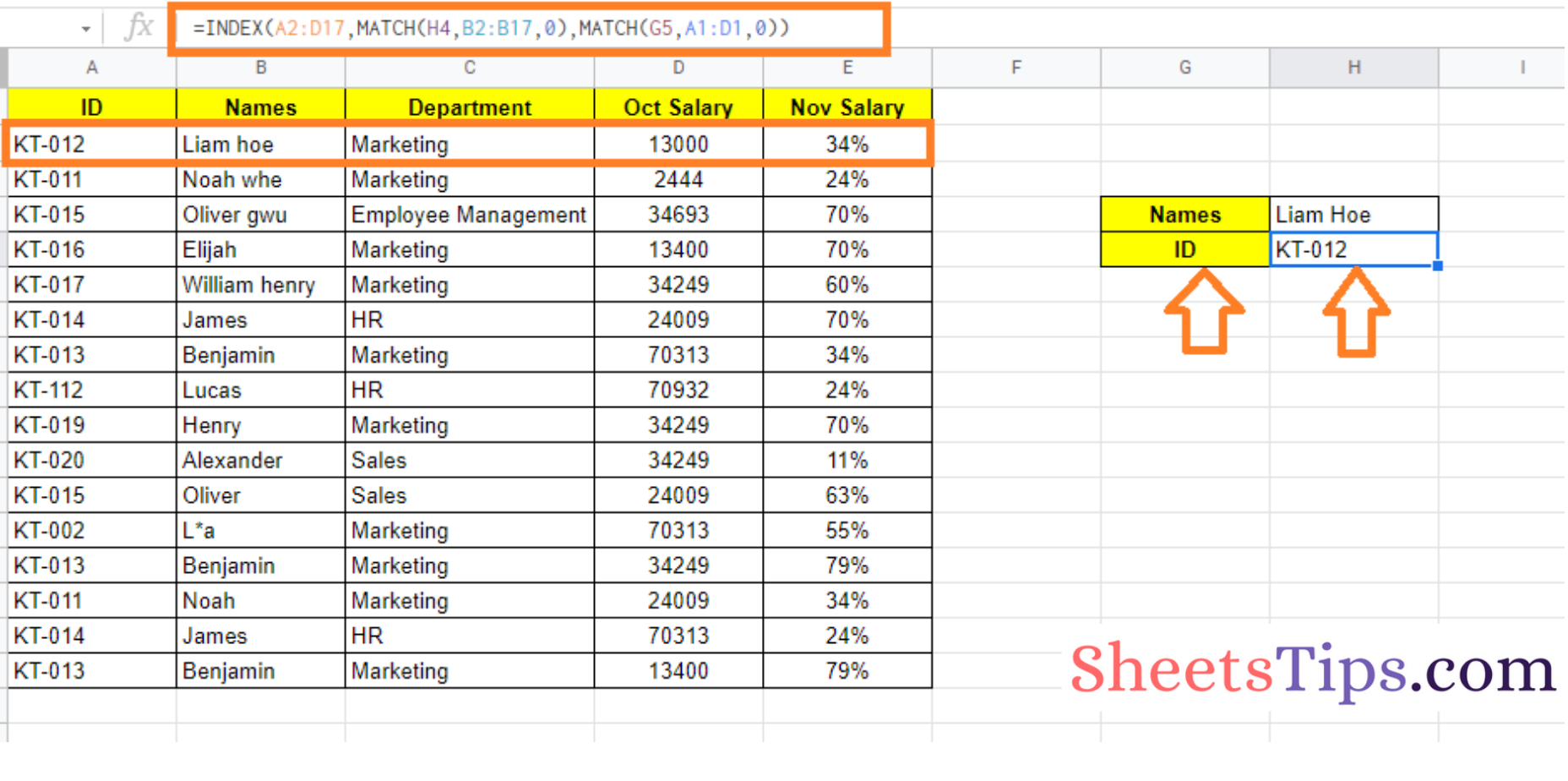
- Step 2: Now type the formula as =INDEX(A2:D17,MATCH(H4,B2:B17,0),MATCH(G5,A1:D1,0)).
- Step 3: Press the “Enter” button.
If cell G6 contains the string “Oct Salary,” as shown below, this formula gives the salary associated with the name specified in cell H4:
This formula provides the monthly ID corresponding to the name specified in cell G6 if cell H4 contains the string “ID”: