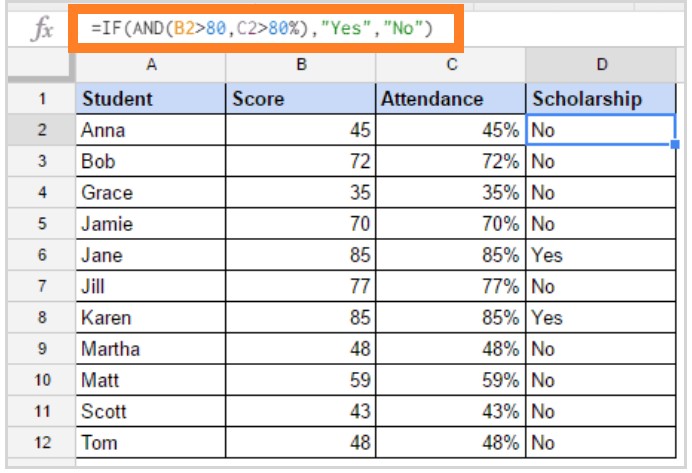
Google Sheets IF Functions: When you want conditions to be checked on the Google sheet, you can use the IF ELSE functions. Usually, the IF function on Google sheets will determine the value and returns True or False based on the conditions set in a particular cell.
For example, let’s consider that we have a student’s scoreboards. Now we will have to check which students have cleared the exams and who got failed in the examination. To check the student’s results status from the scoreboard, we can set IF conditions on Google sheet, which helps us to find which students have cleared the examination and who hasn’t. Let’s understand how to find students results status with the help of the Google sheet tips for IF statement in detail.
How to Insert IF Function on Google Sheets?
One must be aware of IF Statement Syntax, in order to insert IF functions inside the cells of the Google sheet. The Google sheet IF Statement Syntax will contain the following attributes.
IF(logical_expression, value_if_true, value_if_false)
- logical_expression: this is the condition for the function to check. It’s a cell expression that contains a statement that gives a logical value, namely TRUE or FALSE.
- value_if_true: Returns the value if logical statement is TRUE.
- value_if_false: If the conditions are not met and if you don’t specify the statement “value_if_false” argument, then the functions would return “FALSE”. However, this statement is completely optional.
Let’s see some examples of how the IF function can be used in real-life scenarios in Google Sheets.
- Conditional Formatting Based on Another Cell Value in Google Sheets
- How to Extract the Year from Google Sheets-YEAR Function in Google Sheets
- How To Highlight Duplicates In Google Sheets?
Google Sheets IF Statement for Single Condition
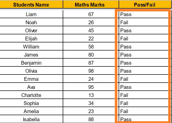
Now we have a students scoreboard and we apply the IF conditions which say that students who secured below 40 marks are Fail and the students who secured above 40 marks are Pass.
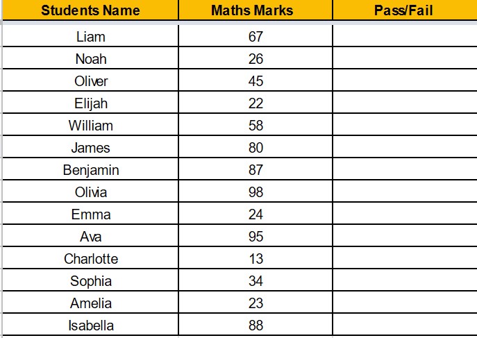
Google Sheet IF Statement Steps:
- Step 1: Select the Cell. Here we are selecting the cell “C2” on the sheet.
- Step 2: Now enter the formula “=IF(B2>40,”Pass”,”Fail”)“.
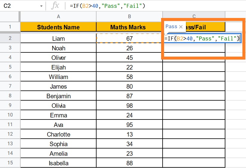
- Step 3: Click “Enter“.
- Step 4: You will see the result.
Google Sheet IF Statement for Multiple Conditions
Using the same example as above, you must chalk up a grading system to a student based on the marks that were made. For example, if the student has secured between 35 to 50, then a D grade should be assigned. Likewise, C grade for the marks between 50 to 70, B grade for 70 to 90, A grade for above 90 and F grade for below 35.
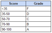
So the multiple IF conditions can be applied on Google Sheet as follows:
- Step 1: Select the “Cell” where you have to apply multiple if conditions.
- Step 2: Enter the formula “=IF(B2<35,”F”,If(B2<50,”D”,If(B2<70,”C”,If(B2<90,”B”,”A”))))“.
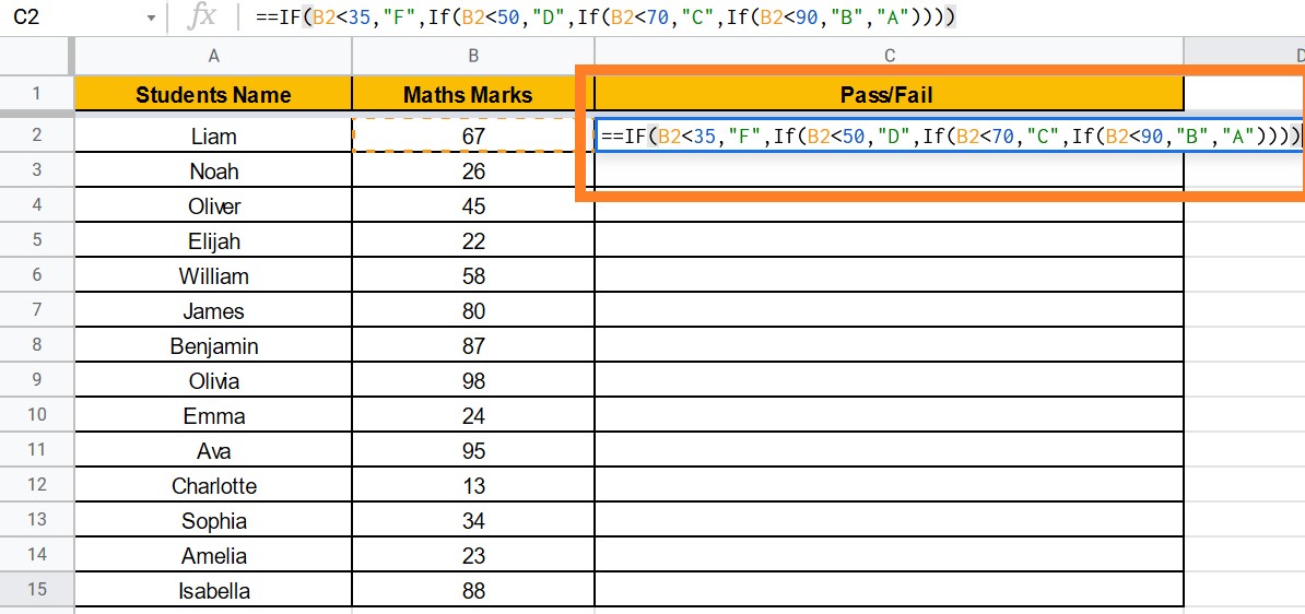
- Step 3: Click on enter. You will see the results.
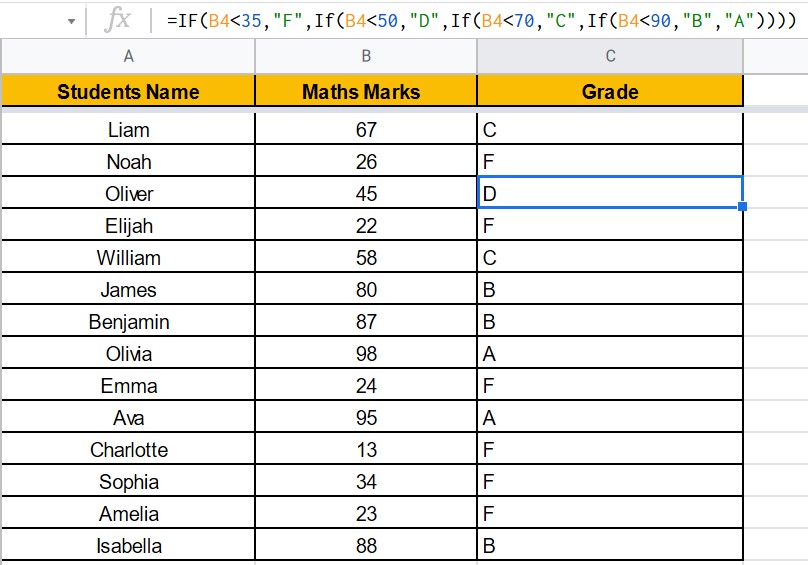
Calculating Commissions Using IF Function in Google Sheets
If Function allows you to calculate in the value section of Google Sheets. The sales commission for sales representatives using the IF function is a good example.
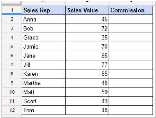
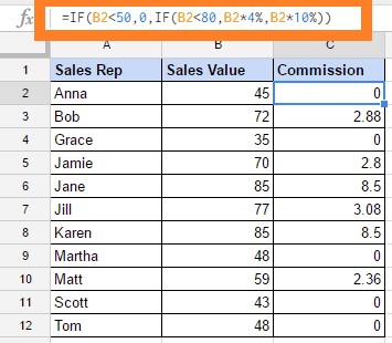
For example, if the sales are less than 50k, a sales representative gets no commission. If the sales are between 50-80k, the salesperson gets 4% commission and 10% if the sales are more than 80k. The following is an illustrative example.
The calculation is carried out within the IF function itself in the formulation used in the example above. When the value for sales ranges from 50 to 100 K, it returns B2*4%, the commission of 4% based on the price.
- Step 1: Select the Cell.
- Step 2: Enter the formula “=IF(B2<50,0,IF(B2<80,B2*4%,B2*10%))“.
- Step 3: Click on “Enter“.
Using And/OR Operators in IF Function
For example, if the sales are less than 50k, a sales representative gets no commission, if the sales are between 50-80k the person will get 4% and 10% if the sales are more than 80k. The following is an illustrative example.
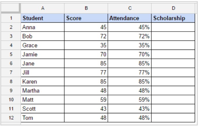
The calculation is carried out within the IF function itself in the formulation used in the example above. When the value for sales ranges from 50 to 100 K, it returns B2*4%, the commission of 4% based on the price.
- Step 1: Select the Cell.
- Step 2: Enter the formula “=IF(AND(B2>80,C2>80%),”Yes”,”No”)“.
- Step 3: Click “Enter“.
