Highlighting Duplicates in Google Sheets: When you’re working on a Google sheet that has numerous duplicate entries, then it would be difficult for you to sort duplicates entries. Manually finding the duplicates and deleting the entries one by one is a time-consuming process. Thus to overcome this, one can make use of the conditional formatting option in Google Sheets which easily highlights and delete the duplicates. On this page, we have provided Google sheet tips and tricks on how to find duplicates and delete them easily in one go. Read on to find out.
How to Find Duplicates in Google Sheets?
Consider you’re already having data set in a column and now you want to find the duplicates for the same. Let’s consider the example of an image given below. Here we will try to highlight the duplicates which are present in Column A. Follow the steps listed below to highlight duplicates in a column.
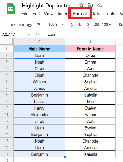
- Step 1: Select the Column A names (excluding headers)
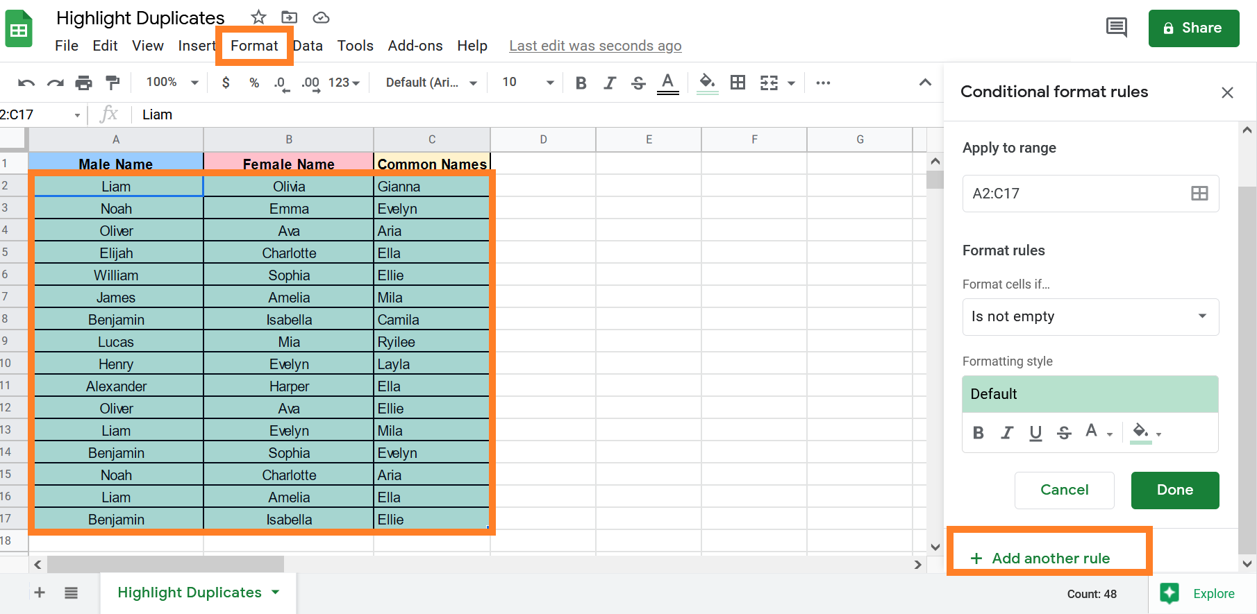
- Step 2: Click on the tab “Format” as shown in the image below:
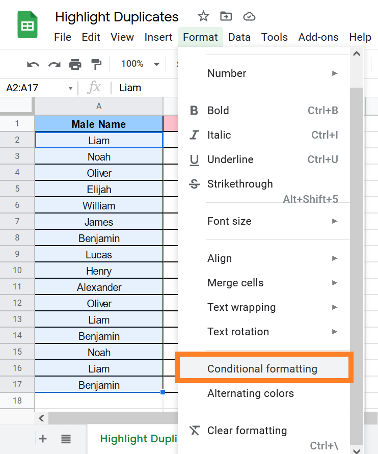
- Step 3: Now clicking on the “Format” tab, select the “Conditional Formatting” from the drop-down menu.
- Step 4: As soon as you click on “Conditional Formatting“, a new tab will open. Here click on “Add another rule” as shown in the image below.
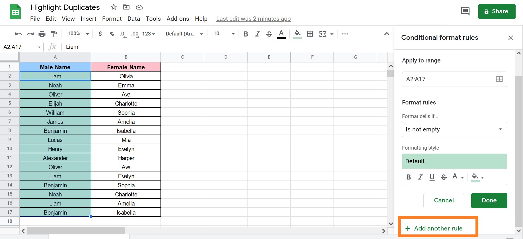
- Step 5: Make sure the range is right (where the duplicates need to be highlighted). If not, you can modify it from the “Apply To Range” section.
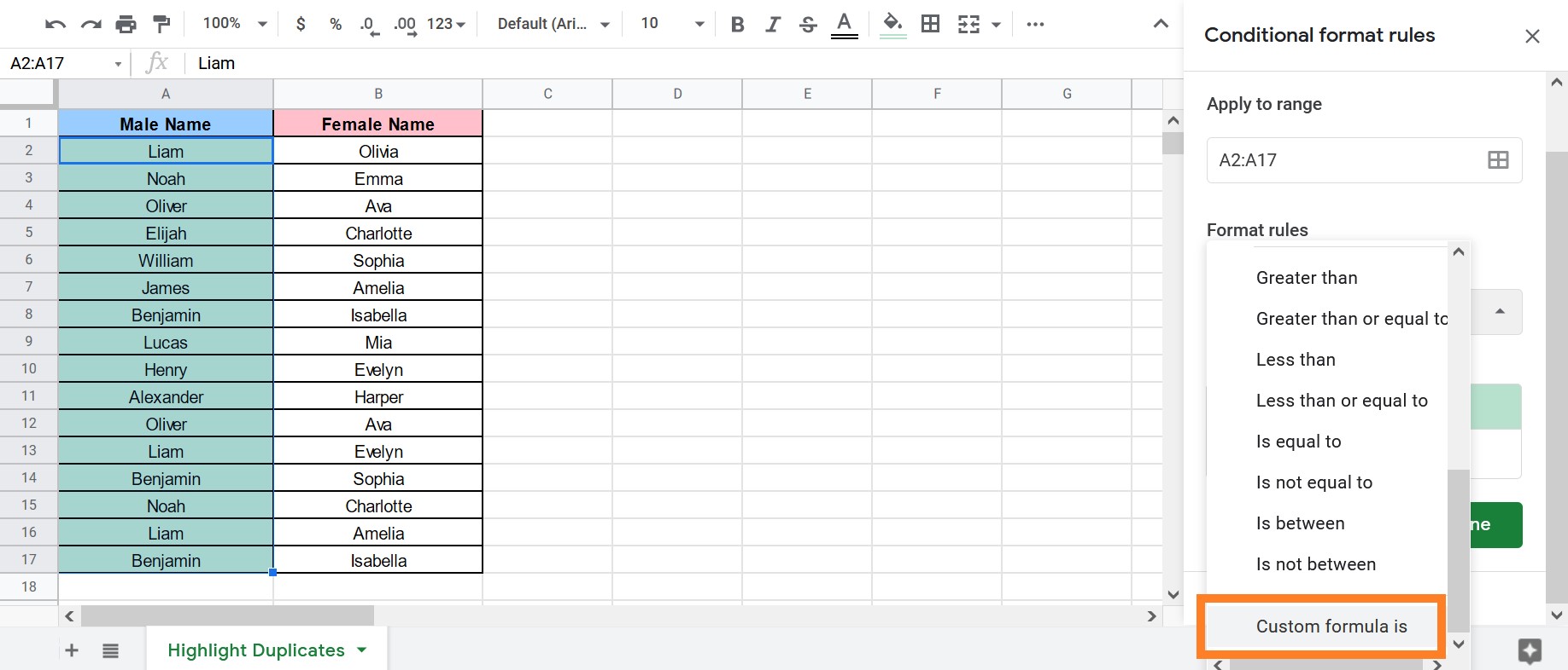
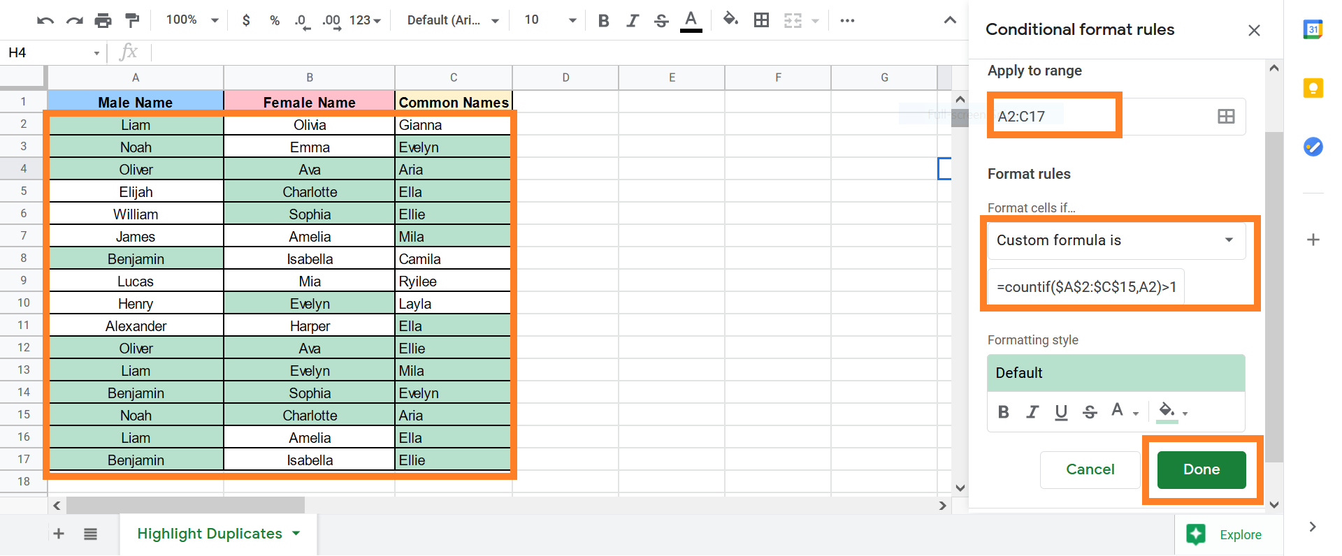
- Step 6: Click the “Custom Formula is” option on the “Format if Cells” button.
- Step 7: Enter the formula “=countif($A$2:$A$15,A2)>1” in the field below:
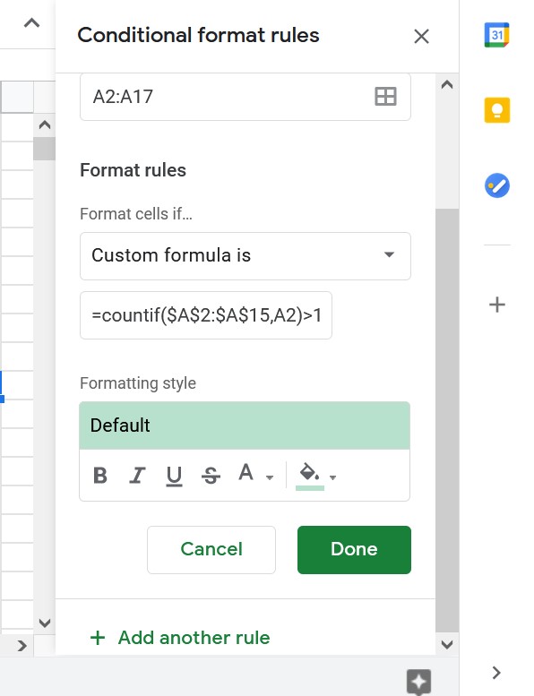
- Step 8: Specify the formatting of the duplicate cells from the “Formatting style” options. By default, green colour is used, but other colours and styles such as bold and italics can be specified.
- Step 9: Click on the “Done” option.
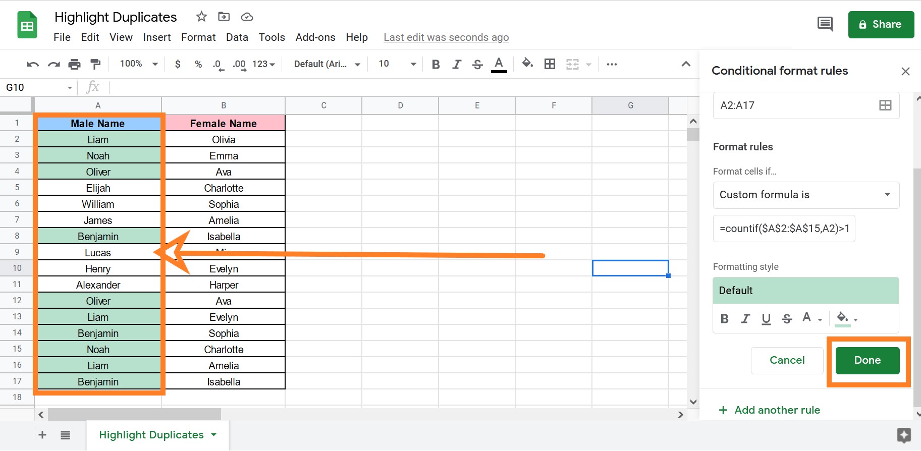
- Step 10: All the cells with duplicate names are highlighted in the colour given as shown below.
How to Highlight Duplicate Cells in Multiple Cells?
We had all the names in a single column in this example. However, what if the names are in several columns?
- How to Remove Duplicates in Google Sheets? (Using Unique Function)
- How to Make an Organization Chart in Google Sheets? – Create an Org Chart in Google Sheets
- How To Insert Indents in Google Sheets? – Know How to Tab Down in Google Sheets
You can still make the duplicate names (which is a name that happens more than once in all three columns combined) via conditional formatting. The steps below explain how to find duplicates in several columns:
- Step 1: Choose dataset names (excluding the headers)
- Step 2: Click on the Format menu option
- Step 3: Click on Conditional formatting from the drop-down menu
- Step 4: Click “add another rule“. Refer to the image below:
- Step 5: Make sure the range is right (where the duplicates need to be highlighted). If not, you can modify it from the “Apply to Range” section
- Step 6: Now click on “Format Rules” and select the “Custom Formula“.
- Step 7: Enter the formula as “=countif ($a$2 : $c$10, a2) > 1“.
- Step 8: Specify the formatting of the duplicate cells from the ‘Formatting style‘ options. By default, green is used, but other colours and styles such as bold and italics can be specified.
- Step 9: Click Done. The sheet will highlight the duplicate entries.
How to Highlight Duplicate Rows/Records?
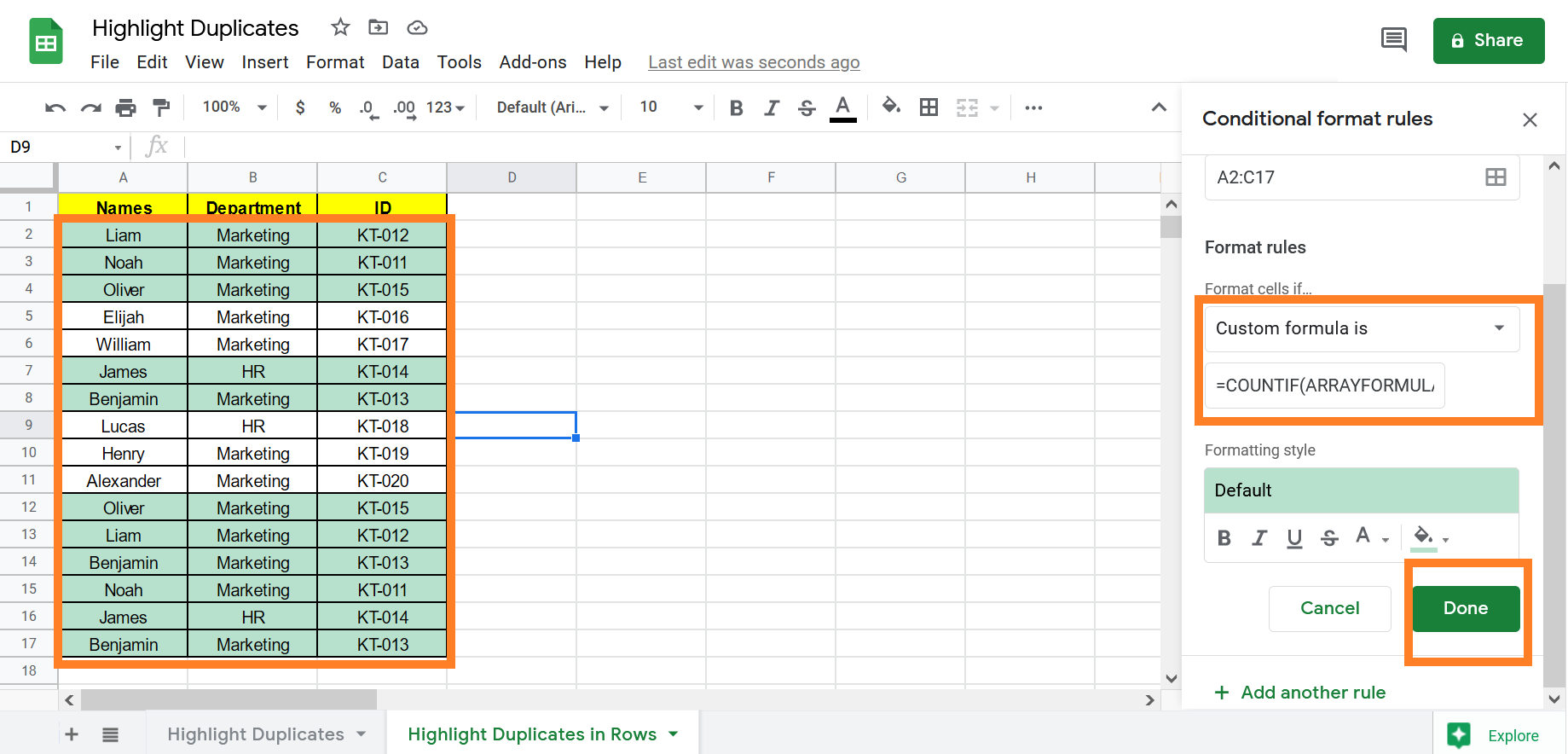
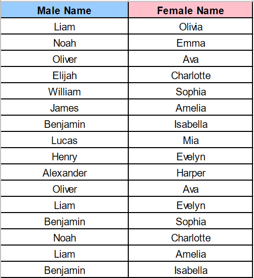
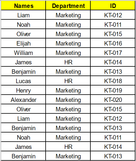
If the value is exactly the same in every cell in the row, the record will be a duplicate and finding the data entries manually will consume a lot of time. For example, you have the following dataset and want the duplicate records to be highlighted, then follow the steps listed after the image to find the duplicate entries.
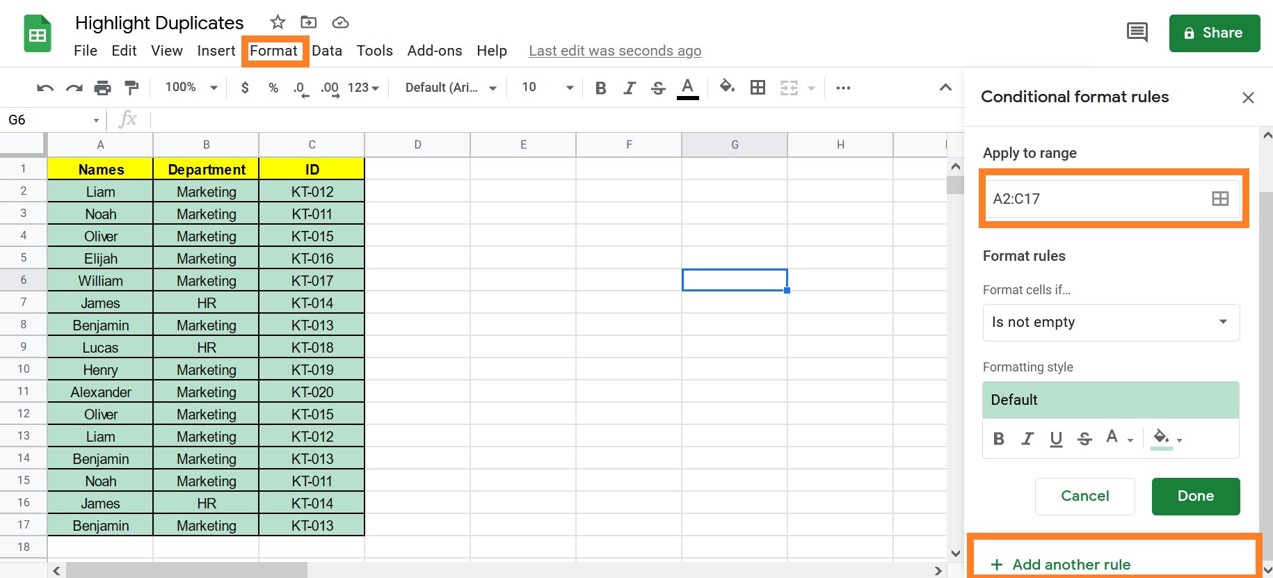
- Step 1: Choose the dataset (excluding the headers)
- Step 2: Click on the Format menu option
- Step 3: Click on Conditional formatting for the options that appear.
- Step 4: Click “Add a different rule“
- Step 5: Click the ‘Custom Formula is‘ option on the ‘Format if Cells‘ button
- Step 6: Now enter the formula as “=COUNTIF(ARRAYFORMULA($A$2:$A$10&$B$2:$B$10&$C$2:$C$10),$A2&$B2&$C2)>1“.
- Step 7: Click on “Done”. The Google sheet will show the duplicate entries.