
Google Sheets are not only used to perform financial or budget analysis operations but also used to perform some fun operations such as reversing text, rotating the text, and so on. Hard to believe right? Yes with the help of Google Sheets, we can perform various operations which are useful for professional and unprofessional purposes. Reversing text is such a feature that is not widely used by every spreadsheet user but when it comes to creating innovative things such as creating quizzes, puzzles, patterns we can use this feature. However, there is no built-in option in Google Sheets like we have text rotation. But still, with the help of formulas, we can simply reverse the texts in Google Sheets.
On this page, let us understand how to reverse the text in a spreadsheet using the Google Sheets Tips. Read further to find more.
Table of Contents |
What is the Formula to Reverse Text in Google Sheets?
The Google Sheets formula to reverse text are is given below:
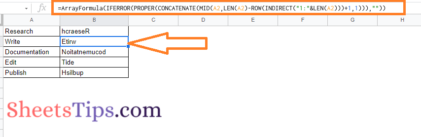
Google Sheets Reverse Formula: =ArrayFormula(IFERROR(PROPER(CONCATENATE(MID(A1,LEN(A1)-ROW(INDIRECT(“1:”&LEN(A1)))+1,1))),””))
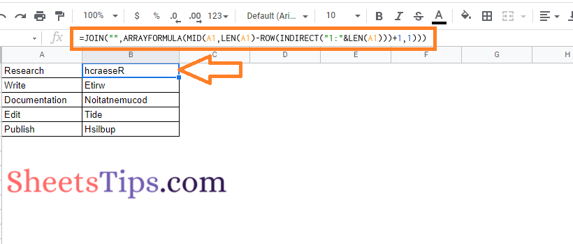
An alternative formula for Google Text Reverse: =JOIN(“”,ARRAYFORMULA(MID(A1,LEN(A1)-ROW(INDIRECT(“1:”&LEN(A1)))+1,1)))
- How To Show Formulas Instead of Values in Google Sheets?
- How to Sync Data From One Google Sheet to Another Spreadsheet?
- How to Add Text Rotation and Perform Accounting in Google Sheets?
How to Reverse Names in Google Sheets with Example?
The step by step to reverse a text or names in Google Spreadsheets are explained below:
- 1st Step: Open the Google Sheets on your device.
- 2nd Step: Now enter the names or the text which you would like to reverse. In our example, we are using column A.
- 3rd Step: Then move to the cell where you want to reverse the entered name or text. In our example, we are using column B to reverse the texts that are entered in column A.
- 4th Step: Now simply enter the formula =ArrayFormula(IFERROR(PROPER(CONCATENATE(MID(A1,LEN(A1)-ROW(INDIRECT(“1:”&LEN(A1)))+1,1))),””)). Here we are using A1 since, it is the column where we want to reverse the text.
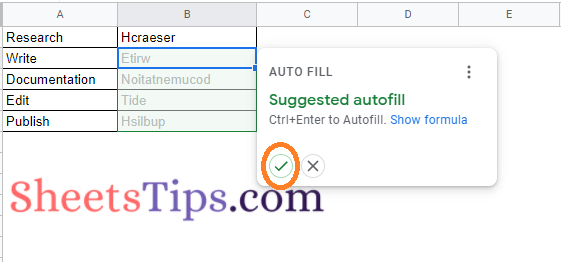
- 5th Step: Press the “Enter” button and you will see the text is reversed. Also now you will have the auto fill feature enabled, click on the tick button to auto fill.
- 6th Step: If it is not enabled, then drag the formula applied cell to other cells using the fill handle and this will simply reverse the text in Google Sheets.
Alternative Formula to Reverse Text
With the help of alternative formula, we can simply reverse the text. Here is another option that also reverses the capitalization.
Working of Reverse Text Formula In Google Sheets
Essentially, we create an array of integers equal to the number of letters in the original text string. Then we reverse the order such that the greatest number appears first in the array. Then each letter in that position is extracted. As a result, the greatest number extracts the final letter, the second largest extracts the second-to-last letter, and so on, until the smallest number extracts the first letter. The separate letters are then concatenated.