
We frequently receive shared Google Sheets in which specific rows or columns are hidden. When the rows are hidden, the user may have the impression that some data is missing. Thus to overcome this, Google Sheets allows us to unhide the rows easily at few clicks. Let’s understand how to unhide rows with important Google Sheet tips. Read on to find out more.
Table of Contents |
How to Unhide Rows in Google Sheets? (For Smaller Dataset)
If you’re looking at a worksheet and something doesn’t seem right, it’s possible that some rows are hidden. As a result, it’s a good idea to look through the sheet for any concealed rows.
Here are some clear clues that your Google Sheet contains hidden rows:
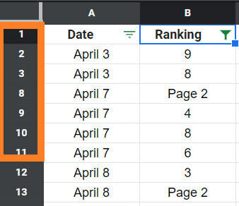
The absence of certain consecutive row numbers is a dead giveaway. Rows 1 to 4 are seen in the image below, and then it skips to row 12. As a result, rows 5 and 11 are hidden.
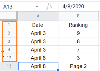
Second, if you carefully examine the rows in your sheet, you should see two arrows on successive rows (as shown below) indicating that there are hidden rows between them.
Steps to Unhide Rows in Google Sheets
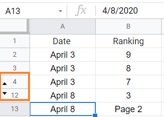
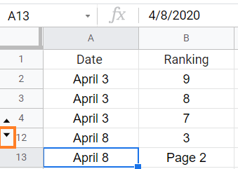
- Step 1: Move the cell where the rows are hidden.
- Step 2: Just click on the “Arrow” button and the hidden rows will be unhidden now.
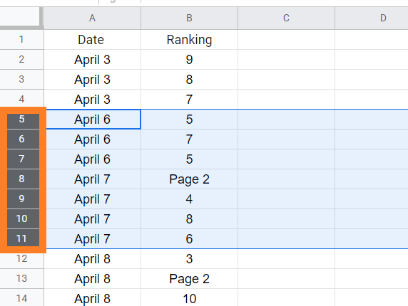
Once the rows are unhidden, the results will be displayed as follows:
- How to Quickly Freeze / Lock Rows in Google Sheets: Freeze or UnFreeze Rows/Columns
- How to Sort by Color in Google Sheets: Multiple Color Sort/Filter by Color
- How to Quickly Transpose Data in Google Sheets: TRANSPOSE, Paste Special Method
Method 2 to Unhide Rows in Google Sheets
The above-explained method is easy. However one can also make use of this method if he/she works with a large number of hidden data. The steps to unhide the data in large numbers are given below:
- Step 1: Select the range of cells, where you feel that data is hidden.
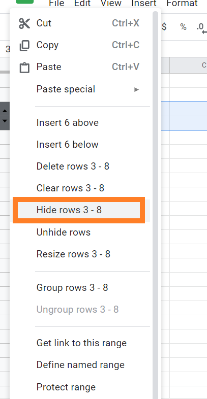
- Step 2: Now simply “Right Click“. A formatting window will be displayed on the screen.
- Step 3: Choose the “Unhide” option. The hidden rows will be now unhidden.
How to Find Rows are Hidden using Filters?
What you think of as “hidden rows” is frequently the result of filters being applied. This is most often the situation when users complain that a few rows are missing but they can’t seem to identify any ‘hidden‘ rows to unhide.
So, here’s how you can tell if a filter is hiding your rows:
- Step 1: In the Filtered applied columns, you will see the Filter icon.
- Step 2: The filter applied rows and columns will appear in different colors.
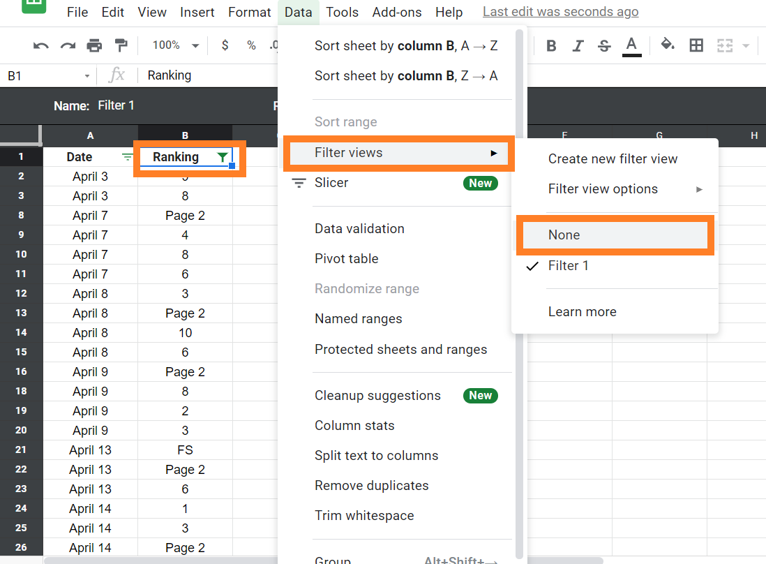
- Step 3: Now click on the Data tab in the menubar.
- Step 4: Select “Filter views“.
- Step 5: Now select “None” from the drop-down menu and the filter will be removed.
On turning off the filter, the rows which are hidden will be unhiding now.
How to Turn Off the Filters in Google Sheets to Unhide Rows?
Simply follow the steps listed below to turn off the filters in Google Sheets:
- Step 1: In the menubar, click on the Data tab.
- Step 2: Click on “Turn Off Filter“. The filter will be turned off if you select “Turn off Filter.”
A Simple Method to Turn off Filter in Google Sheets
The simple method to turn off the filter are explained below:
- Step 1: Click on the “Filter” icon.
- Step 2: From the drop-down menu, click on “None“.
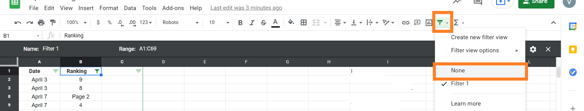
The filter will be removed and the rows which were hidden will be now unhidden.