
Google Sheets Freeze feature can be used when you have a huge number of data that needs to be scrolled up and down. With the help of the Google Sheet Freeze function, you freeze both the rows and columns. Basically, the Freeze function freezes the top rows/columns that would make these rows/columns constantly visible even while scrolling the cell up and down.
On this page, let’s understand how to freeze or lock the rows along with important Google Sheet Tips. Read on to find more.
Table of Contents |
Methods to Freeze Rows in Google Sheets
There are namely 2 easy methods with the help of which we can easily freeze the rows or columns in Google Sheet. The list of methods which is used to freeze the rows and columns in Google Sheet is given below:
- Using Mouse or keypad
- Using Menu Options
Google Sheets Freeze Rows using Mouse or Keypad (Shortcut)
The steps to freeze the rows with the help of a mouse or keypad are explained below:
- Step 1: Decide the number of rows that you would like to freeze.
- Step 2: Now just drag the dark grey line to the rows you would like to freeze.
- Step 3: Till the grey line is dragged, the rows will be frozen as shown below.

Freeze Columns using Mouse or Keypad in Google Sheet
In order to freeze or lock the columns, just follow the same steps which are used to freeze the rows in Google Sheets.
- Step 1: Decide the number of columns you would like to freeze.
- Step 2: Now just click on the dark grey line to the column you have decided to freeze.
You will see the results as follows.

- How to Set Print Area in Google Sheets: Page Setup, Print Layout in Google Sheets
- Jump To Cell Range in Google Sheets – How To Jump To Specific Cell Range in Google Sheets?
- How to Quickly Transpose Data in Google Sheets: TRANSPOSE, Paste Special Method
Freeze Rows using Menu Options in Google Sheet
This method is time-consuming, however, this method will be a great help if you have any issues selecting the cells by dragging the mouse or keypad.
- Step 1: Select the number of rows you would like to freeze.
- Step 2: Click on “View” and select “Freeze” from the drop-down menu.
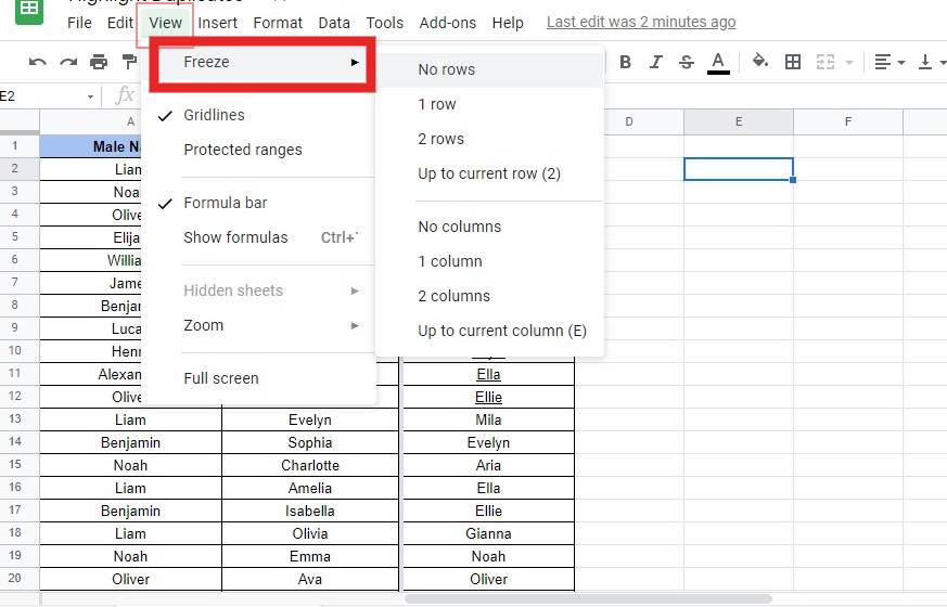
- Step 3: As soon as you click on the Freeze button, you will be provided with options.
- Step 4: Select the number of rows to freeze the cells and the selected cells will be frozen.
Freeze Columns using Menu Options in Google Sheet
Follow the steps listed below to freeze the columns using the menu option.
Step 1: Go to the Google Sheets Menu bar.
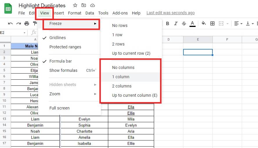
Step 2: Click on “View” and select “Freeze“.
Step 3: Now go to the Columns section and select the number of columns that need to be frozen.
You will see the results as shown below.
How to Unfreeze Rows or Columns in Google Sheets?
You can unfreeze rows or columns in Google Sheets by following the steps listed below:
- Step 1: Select the cell which are frozen
- Step 2: Click on View and select Freeze.
- Step 3: Select No Rows to unfreeze rows.
- Step 4: Select No columns to unfreeze columns.
The selected rows or columns will be unfreezed now.