Hyperlinks in Google Sheet Cells: Hyperlinks help us to navigate the user from one to another page. Usually, the hyperlinks are commonly seen on Web pages. However, Google Sheets also allows using the text with hyperlinks with the help of which users can navigate from page to page.
Let’s understand how to create and edit hyperlinks with the Google Sheet tips provided on this page.
How to Add a Hyperlink to a Google Sheet?
We can add hyperlinks to Google Sheets with the help of any of the following two methods such as:
- Using Insert Menu
- Using Hyperlink Formula
Adding Hyperlinks to Google Sheets using Menu Option
The steps to add hyperlinks to the Spreadsheet using the menu option are explained below:
- Step 1: Select the cell where you want to create a hyperlink.
- Step 2: Now click on the “Insert” menu and select “Link” from the drop-down menu.
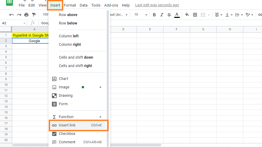
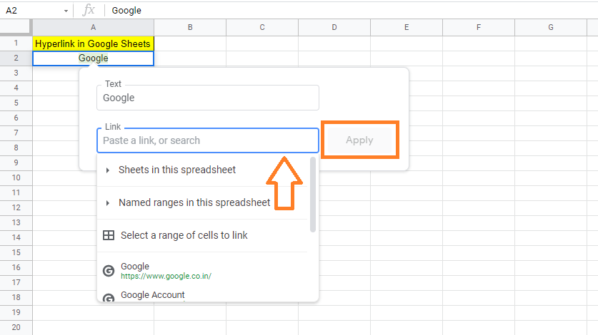
- Step 3: A dialog box opens on the screen. Paste the URL and press Apply button. The hyperlink is created.
Using Google Sheets Hyperlink to Cell Formula
We can also create a hyperlink to desired text by following the steps listed below:
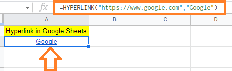
- Step 1: Select the cell.
- Step 2: Now enter the formula as HYPERLINK(URL, LINK_LABEL). In the URL part, paste the URL, and in the Link_Label Part, enter the text for which the hyperlink should be created.
- Step 3: Press the “Enter” button. You will see the results.
- How to Create a Drop Down List in Google Sheets: Add/Remove/Customize Drop Down Menu
- How To Insert Indents in Google Sheets? – Know How to Tab Down in Google Sheets
- How to Color Alternate Rows in Google Sheets: Alternating Colors Every 2 Rows, 3 Rows
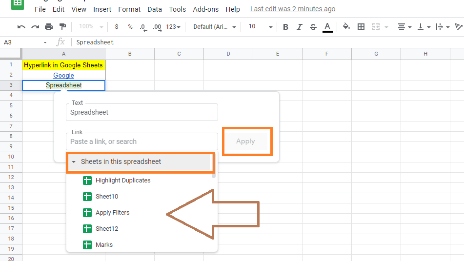
Hyperlink to Another Sheet in Google Sheets
We can also hyperlink another Google Spreadsheet in this Google Sheet. The steps to hyperlink another sheet in Google Sheets are explained below:
- Step 1: Select the cell where you want to insert the hyperlink.
- Step 2: Now click on the “Insert” tab and select “Link” from the dropdown.
- Step 3: Then select Sheets in this spreadsheet option from the hyperlink dialog box.
- Step 4: Now under the link option, type the sheet name.
- Step 5: Here a list of sheets with a similar name will open on the screen. Now select the sheet name and click on “Apply“.
- Step 6: The hyperlink will be applied.
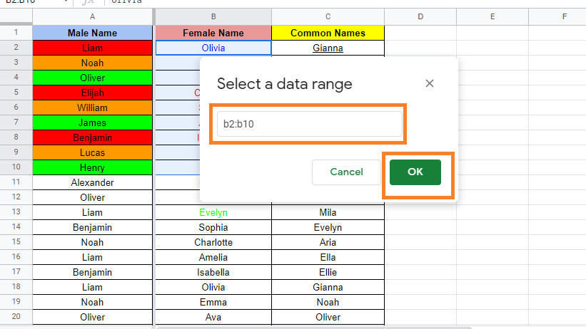
Bulk Hyperlink in Google Sheets
We can also apply hyperlinks to a range of cells in Google Sheets by following the steps listed below.
- Step 1: Select the cells to insert the hyperlinks.
- Step 2: Now go to the “Insert” option and select “Insert link.“
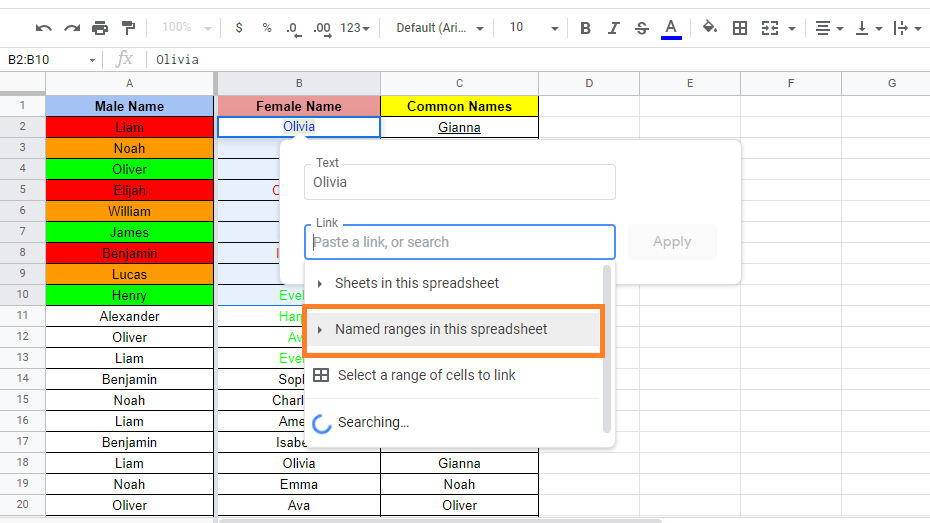
- Step 3: Hyperlink dialog box opens on the screen. Now choose to Select a range of cells to link from the options.
- Step 4: Now enter the cell range and specify the URL to be linked.
- Step 5: Click on the “Apply” button and the hyperlinks will be applied to the selected range of cells.
<h3id=”Keyboard-Shortcut-to-Insert-Hyperlink”>Keyboard Shortcut to Insert Hyperlink
The keyboard shortcut to insert the hyperlinks in Google Sheets are explained below:
- Step 1: Select the cell where you want to insert the hyperlink.
- Step 2: Double click the cell to edit and select the text to link.
- Step 3: Now press “Cntrl+K“.
- Step 4: The hyperlink dialog box will open on the screen.
- Step 5: Now paste the URL and click on “Apply“.
The hyperlink will be inserted into the desired cell.
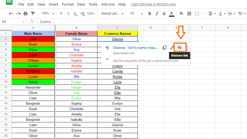
How to Remove Hyperlink in Google Sheets?
To remove the hyperlink in Google Sheets, follow the steps as listed below:
- Step 1: Select the cell where you want to remove the hyperlink.
- Step 2: Now click on the “Remove hyperlink“.
- Step 3: The selected text’s hyperlink will be removed.
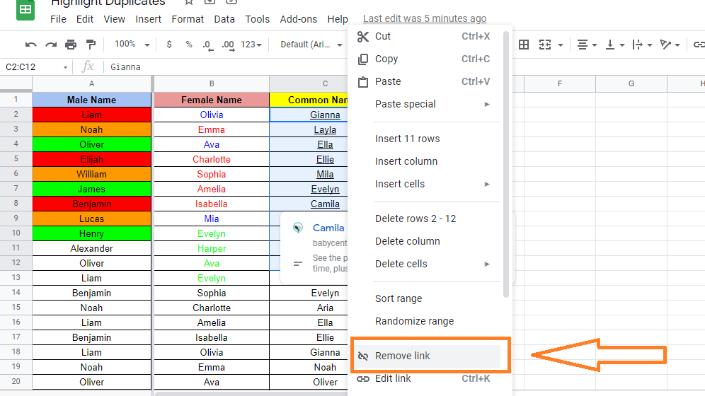
How to Remove Hyperlink in Google Sheets in Bulk?
To remove the hyperlink in bulk, follow the steps as listed below:
- Step 1: Select the range of cells where you want to remove the hyperlink.
- Step 2: Now right-click and move the “Remove Link“.
- Step 3: Click on it. The hyperlink will be removed.