Adding dynamic bands to your Google Sheets is very useful to highlight specific parts of the chart. Using simple formulas, we can easily create the dynamic bands for the charts on Google Sheets. On this page, let us discuss how to create the dynamic chart banding in the spreadsheet using Google Sheets Tips and Tricks. Read further to find out more.
| Table of Contents |
Creating Dynamic Chart Bands in Google Sheets
To create a dynamic band for the charts in Google Sheets, we will have to create the dataset. In this post, I have used the Website Traffic analysis dataset and have modified the same as follows.
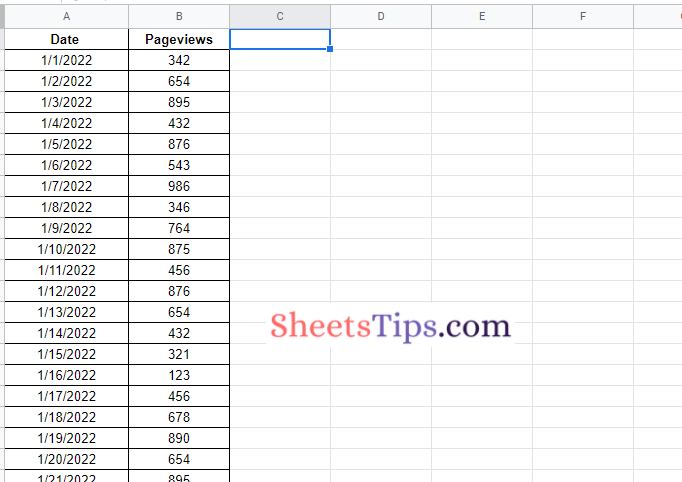
As shown in the image above, I have dates and pageviews in Columns A and B.
- How to Create a Gantt Chart in Google Sheets? (Dynamic Gantt Chart Formula)
- Radial Bar Chart in Google Sheets Example – Learn How To Make Radial Chart in Spreadsheet
- How to Create a Grid Chart in Google Sheets? – Add Grid Lines and Borders in G-Sheets
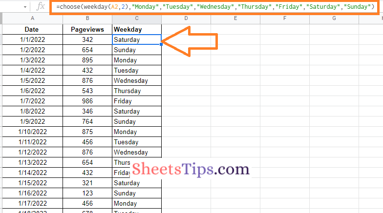
Now in Column C, we will have to determine whether the specified date in Column A falls on which weekday. To analyse the same, we are using the formula “= choose (weekday (A2, 2), “Monday”, “Tuesday”, “Wednesday”, “Thursday”, “Friday”, “Saturday”, “Sunday”)“. Once you enter this formula, you will have the results as follows:
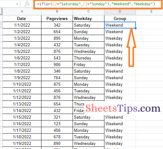
The next step is to know if the days in column C fall on a weekend or a weekday. To find out, we use the following formula:
=if(or(C2="Saturday",C2="Sunday"),"Weekend","Weekday")
This formula categorizes the day as a weekday or weekend as per the calendar. So your results will be as follows:
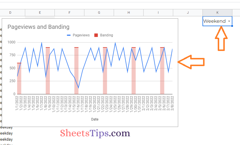
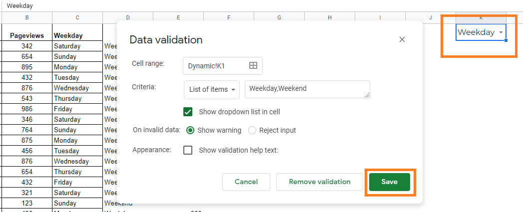
Finally, we need to create a data validation drop-down list for weekdays and weekends. In this post, I have chosen Column K to create the data validation as shown in the image below.
Now in Column E, we are creating the banding. So our formula in Column E is “if (D2=$K $1,900,””)“. Press the “Enter” key and you will see the results as shown below.
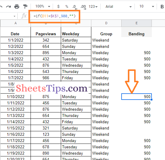
So our dataset will finally look like the above image.
How to Make a Dynamic Chart Banding in Google Sheets?
The steps for creating dynamic chart bands in a Google Spreadsheet are as follows:
- 1st Step: Select Columns A, B, and E in the above dataset.
- 2nd Step: Click on the “Insert” tab and choose “Chart” from the drop-down menu.
- 3rd Step: By default, Google Sheets will create a chart.
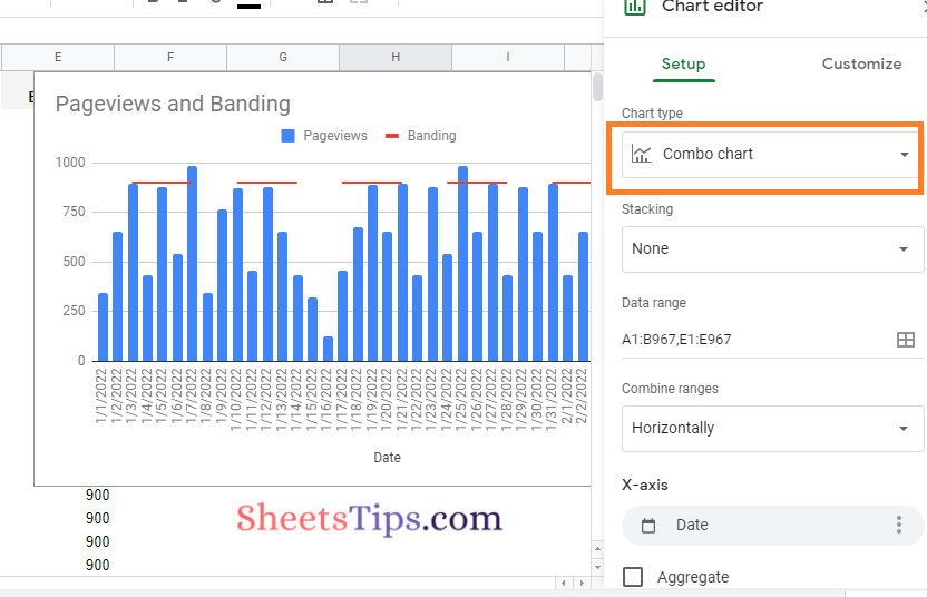
- 4th Step: Now select “Combo Chart” under the Chart Type.
- 4th Step: Now we have to customise the combo chart. To do the same, click on the “Customise” section.
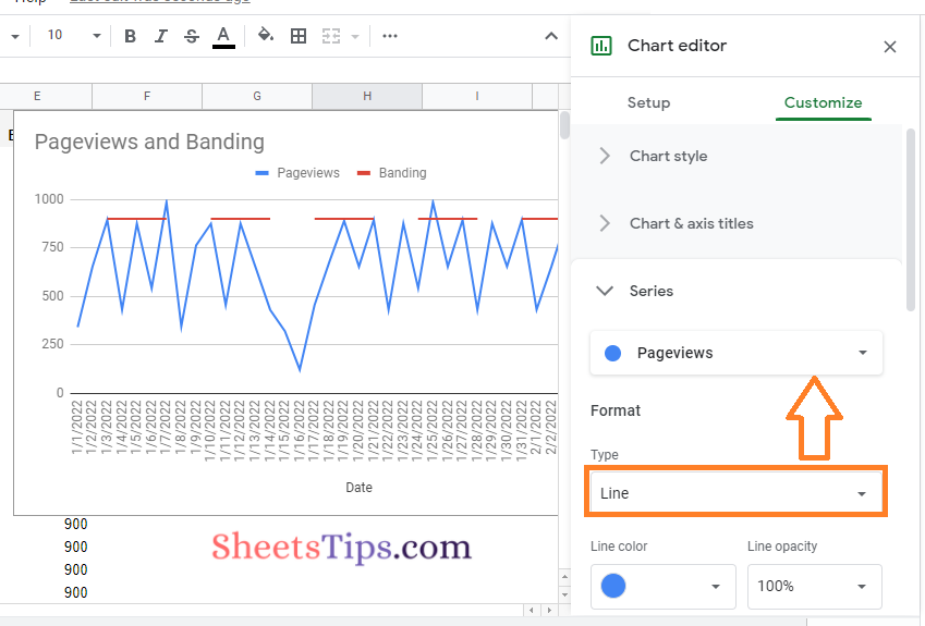
- 5th Step: Under “Series,” select “Page Views.”
- 6th Step: Select “Type” as lines.
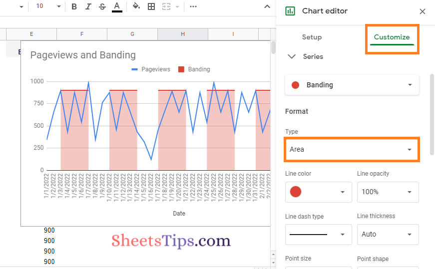
- 7th Step: Now again, under “Series“, choose “Banding” and select the “Type” as “Rows“.
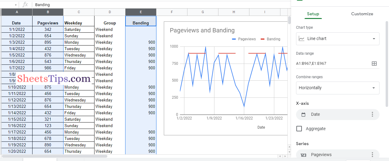
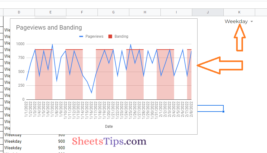
- 8th Step: That’s it. The Dynamic Band Chart has been created. Now in column K, choose the “Weekday” from the drop-down list and you will see the following results.
Changing the drop-down list to “Weekend” will help you see the following results.