Slicers in Google Sheets are an effective tool for filtering data in Pivot Tables. With a single click, they make it simple to change values in Pivot Tables and Charts. Slicers come in handy when creating dashboards in Google Sheets. In this article, let us understand how to use Slicer in Pivot tables with the help of Google Sheet tips provided on this page. Read on to find more.
Table of Contents |

Slicers in Google Sheets
Consider the following dataset. It consists of a small pivot table.
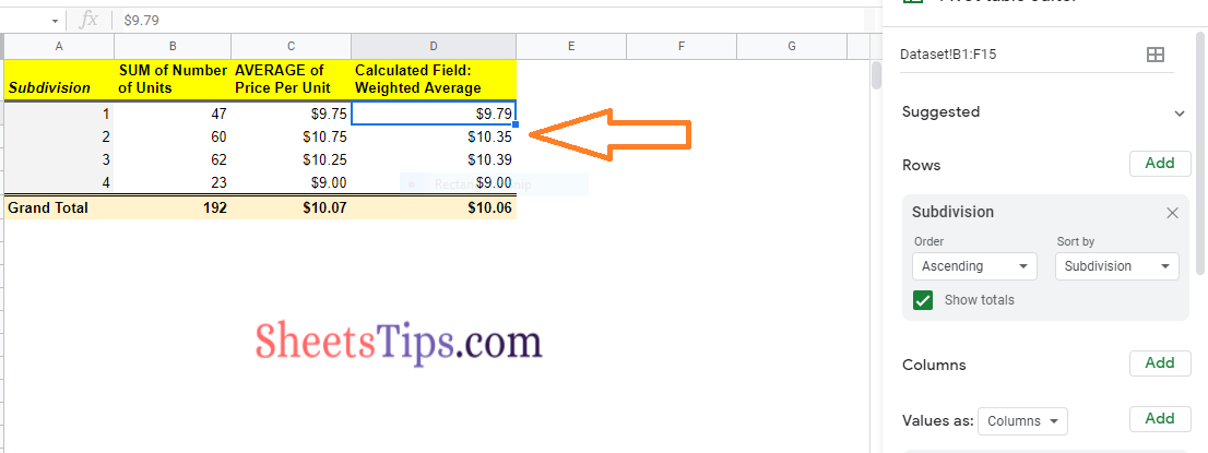
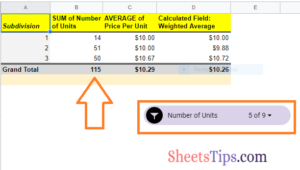
Now in the same dataset, you can see the slicer being created. When you modify this slicer filter, the pivot table will be modified.
- How to Group by Month in Pivot Table in Google Sheets (With Examples)
- How to Add & Use Calculated Fields in Google Sheets Pivot Tables
- How to Insert a Pivot Table in Google Sheets? (Create/Edit/Customize Pivot Tables)
How to Add Slicer in Google Sheets?
The steps to create a slicer in Google Sheets are given below:
- Step 1: Open a spreadsheet on your computer by going to sheets.google.com.
- Step 2: Click on the dataset to open the Pivot table. Check our article on how to insert a pivot table, if you haven’t created a pivot table in Google Sheets.
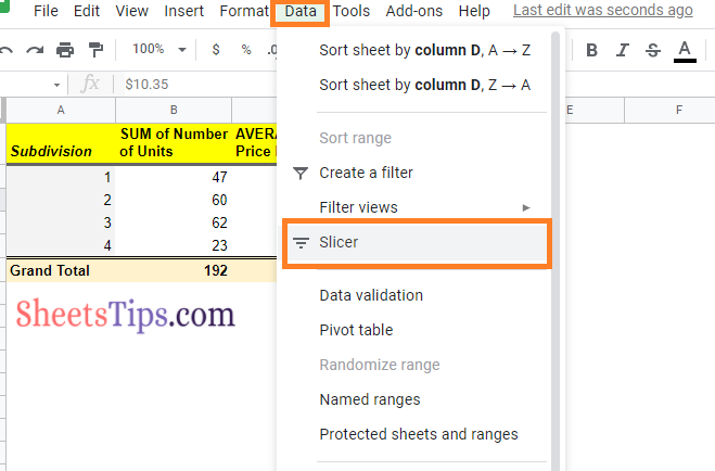
- Step 3: At the top, select Data, followed by Slicer.
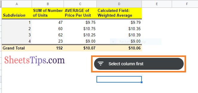
- Step 4: Select a column to filter by on the right.
- Step 5: Select your filter rules by clicking the slicer. Here you will be provided with 2 options and they are:
- Filter by Condition: Select from a list of predefined conditions or create your own.
- Filter by Values: Uncheck any data points you want to hide.
Now you will see the slicer being created on Google Sheets as shown below:
How to Edit Slicer in Google Sheets?
By default, the Slicers will show up in Black color. In order to edit or customize the slicers in Google Sheets, follow the steps as listed below:
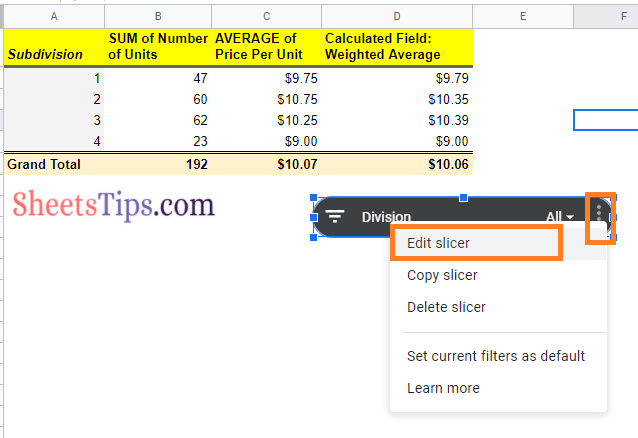
- Step 1: Click on the Slicer being created on the Google Sheets.
- Step 2: Now click on the 3 dots and select “Edit Slicer“.
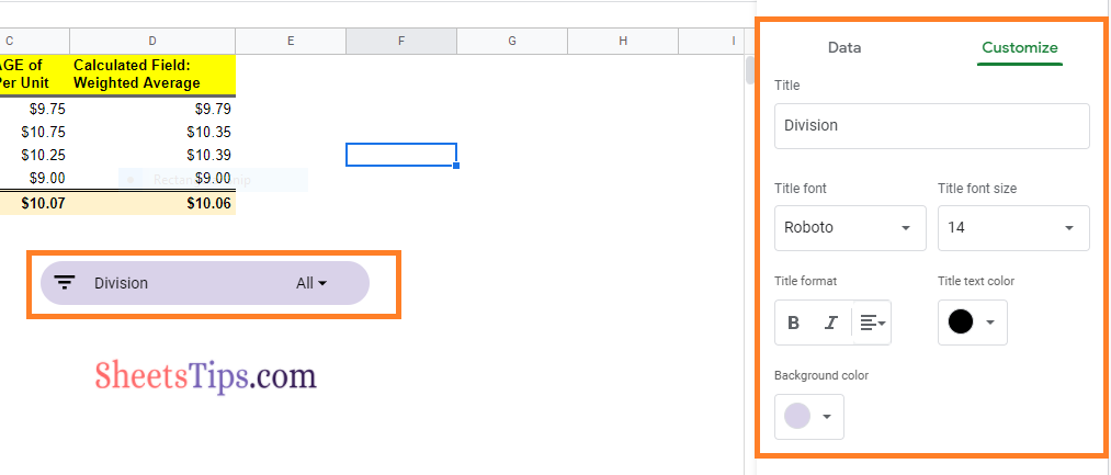
- Step 3: Here a window will open on the screen. Here you will be provided with various options.
- Step 4: To change the Title of the Slicer, modify the Title in the Title window.
- Step 5: You can change the Title font and its size by moving to its respective window.
- Step 6: Click on the “Title Text Color” window to change the title color.
- Step 7: To change the title background color, make the necessary changes in the background color window. In this article, we have customized our Slicer in Google Sheets as shown in the image below:
How to Interact with Slicers in Google Sheets?
Now let us understand how to interact with Slicers in Google Sheets by following the steps as listed below:
- Step 1: Click on the “All” drop-down menu in the Slicers.
- Step 2: Here you will have two options – Filter by condition and Filter by value.
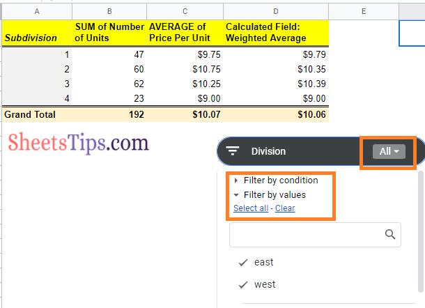
- Step 3: Now select how the data needs to be filtered.
- Step 4: Click on the “Ok” button and you will see the data being filtered in the Pivot table.
How to Delete Slicers in Google Sheets?
The steps to delete the Slicers in Google Sheets are given below:
- Step 1: Click on the Slicers.
- Step 2: Press the “Delete” button or “Backspace” button. Else click on the 3 dots and choose “Delete Slicer” to delete the slicers.
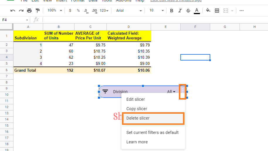
The slicers will be deleted.