
Google Sheets comes with n number of features. Of all, one of the important features of Google Sheets is that we can compare two columns to find the difference or exact data. However, we will need to enter the formula manually to compare the columns in Google Spreadsheet. In this article, we have provided few Google Sheet tricks where you can easily compare two columns and get the desired results. Read on to find out more.
Table of Contents |
How to Compare Two Columns in Google Sheets?
Follow the steps listed below to compare the two columns in Google Sheets.
- Step 1: Make sure you have the data set in Column 1 and Column 2.
- Step 2: Move to Column 3 to enter the formula. Now enter the formula as “=Column 1 = Column 2“. (The column represents the cell name).
- Step 3: In our case, the formula is =A2=B2. Now press the “Enter” button.
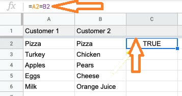
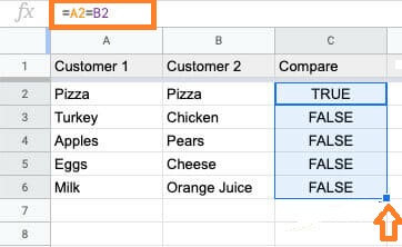
- Step 4: It returns True if the value/data is matched. If not the cell returns False. Drag the formula applied cell downwards to apply the same formula.
How to Make a Conditional Comparison across Two Columns?
Comparing two columns doesn’t only limit to it. We can use conditional operators to make comparisons and check the results based on them. Follow the steps listed below to make the comparison using conditional operators.
- Step 1: Double-check that the data set is in Columns 1 and 2.
- Step 2: To enter the formula, go to Column 3. Enter the formula as =IF(Conditional Statement (<, >, =, etc),”Cell 1 True Text”,”Cell 2 True Text”).
- Step 3: Press “Enter“. You will see the results.
For example, we have the following dataset and want to compare the marks and return the value as “High” and “Low”. So our formula will be =IF(A2>B2,”High”,”Low”).
- How To Insert Indents in Google Sheets? – Know How to Tab Down in Google Sheets
- Funnel Charts In Google Sheets – How To Make Funnel Templates In Google Spreadsheet?
- How to Make an Organization Chart in Google Sheets? – Create an Org Chart in Google Sheets
Comparing Two Columns to Find Highest & Lowest Values
We can also compare two columns to find the highest and lowest values. The steps to perform this operation are explained below:
- Step 1: Make sure you have the dataset in two columns and move the column where you would like to see the results.
- Step 2: In the cell, write the formula =max(range start: range end).
- Step 3: Press the “Enter” button. You will see the results.
In our case, we are using the formula max(A2:B2). To find the minimum value, we can use the formula min(A2:B2)
Compare Two Columns to Find Matching Data
Follow the steps listed below to find the matching data in Google Sheets.
- Step 1: Select the cells where you want to find the matching data.
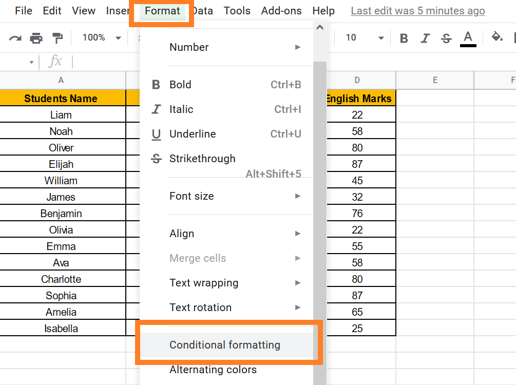
- Step 2: Click on the “Format” menu and select “Conditional Formatting” from the drop-down menu.
- Step 3: The ‘Conditional format rules’ sidebar will appear on the right side of the window. Type the range of cells you want to apply the formatting to in the input box under “Apply to the range.“
- Step 4: Then, under “Format cells if,” select the dropdown arrow in the Format rules section.
- Step 5: Select “Custom formula is” from the selection menu that opens. Now type the formula as ” =COUNTIF($A$2:$A$9,B2)>0“
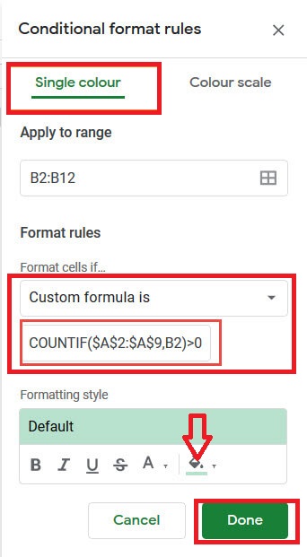
- Step 6: Under “Formatting Style” select the Fill color to highlight the data.
- Step 7: Click on “Done“. You will see the results.
Compare Two Columns to Find Missing Data
The steps to compare two columns and find the missing data are explained below:
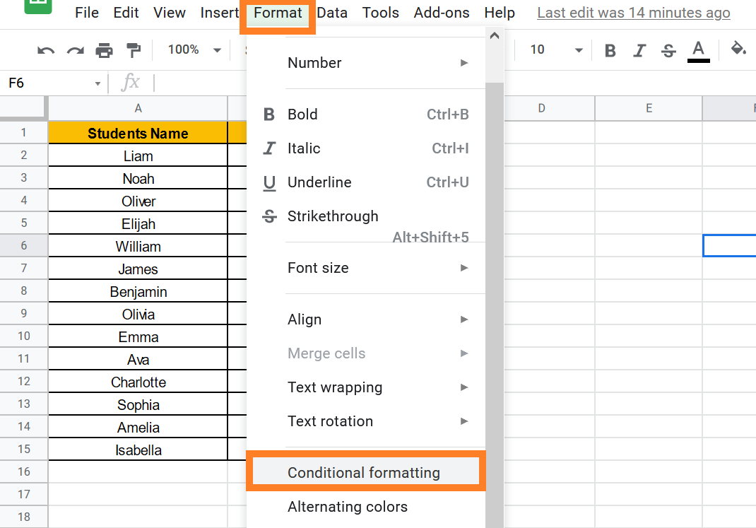
- Step 1: From the menu bar, select the Format option.
- Step 2: Choose ‘Conditional Formatting‘ from the drop-down menu.
- Step 3: Type the range of cells you want to compare in the input box under “Apply to range.” We can type A2:B12 in our example.
- Step 4: Then, under “Format cells if,” select the dropdown arrow in the Format rules section.
- Step 5: Select “Custom formula is” from the selection menu that opens.
- Step 6: Below the dropdown list, you’ll see an input box. Enter “=COUNTIF($A$2:$A$9,B2)=0” as your custom formula.
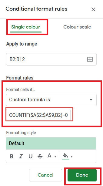
- Step 7: Click the Fill Color button under “Formatting style.” and select the Fill color.
- Step 8: Press the “Done” button. You will see results.