Google Sheets Funnel Charts are one of the most useful charts that help to understand the data more easily just by seeing it. However, to create funnel charts in Google Sheets, one will have to either use tools such as funnel chart maker or funnel chart creator. Yet, not to worry because, on this page, we have provided a technique with the help of which you can easily devise funnel charts in Google Sheets. Using the Google Sheets Tips provided on this page, one can easily create a funnel chart without using code and additional add-ons. Read further to find out more.
Table of Contents |
How Do You Make Funnel Charts in Google Sheets?
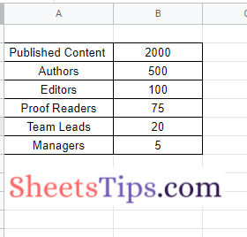
In order to construct a funnel chart in a Google Spreadsheet, one will have to create a dataset. For this post, I have created an example dataset as follows:
Firstly, I am listing down the number of people working in publishing houses and dividing them according to their departments. So the first two columns of my dataset are as follows:
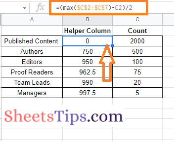
Secondly, I am creating a helper column. To create a helper column, I am using Column C and my helper column formula is “".
- How to Create Leave Tracker Template in Google Sheet (Free Leave Tracker Template Download)
- How To Sync Charts From Google Sheets to Google Docs & Google Slides?
- How to Create a Grid Chart in Google Sheets? – Add Grid Lines and Borders in G-Sheets
Entering the above formula will show the following results in Google Sheets. Now our dataset is ready, let us start by creating a funnel chart in Google Sheets in the next section.
How Do I Add Funnel Charts to Google Sheets?
The steps to inserting a funnel chart in Google Sheets are as follows:
- 1st Step: Select the dataset that we have created on Google Sheets.
- 2nd Step: Click on the “Insert” tab in the menubar and choose “Chart” from the drop-down menu.
- 3rd Step: By default, Google Sheets will create a chart on the spreadsheet. Now double click on the chart to customise the chart.
- 4th Step: Under “Chart Type,” choose “Stacked Bar Chart” from the options.
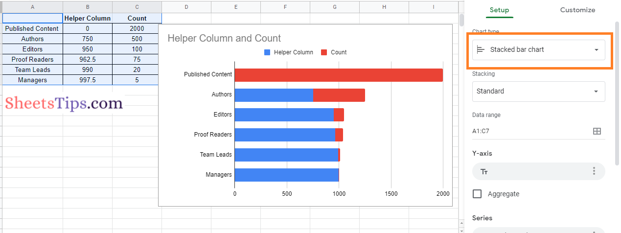
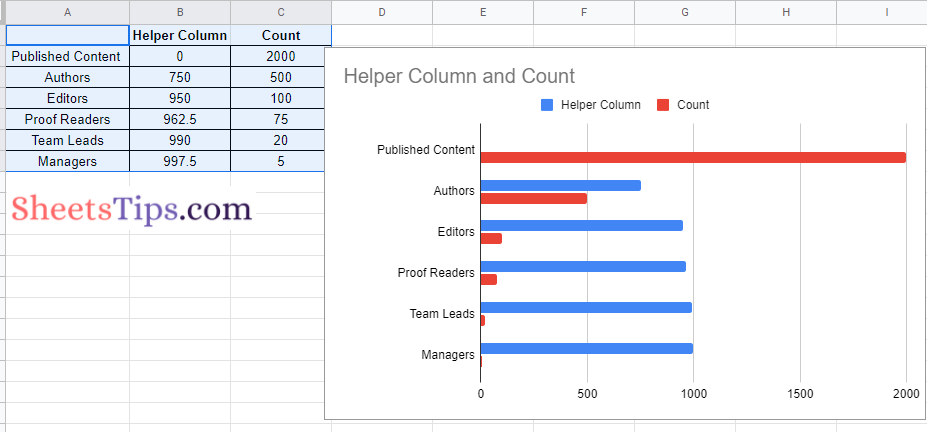
- 5th Step: The Stacked Bar Chart will be generated on Google Sheets. Now customise the Stacked Bar Chart. Under the series, choose “Helper Column“.
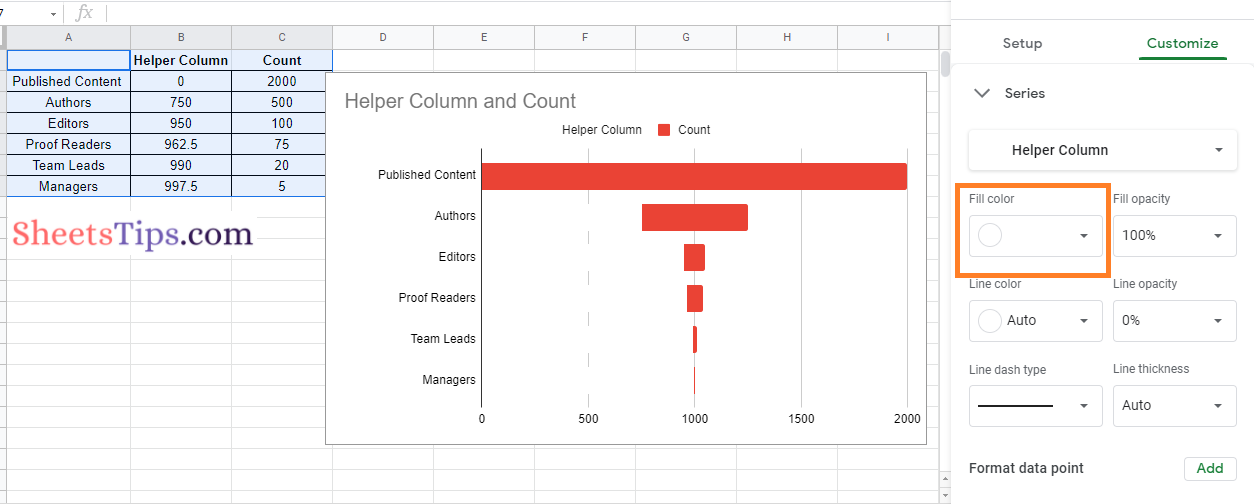
- 6th Step: Set the “Helper Column” colour to white or transparent, as shown in the image above.
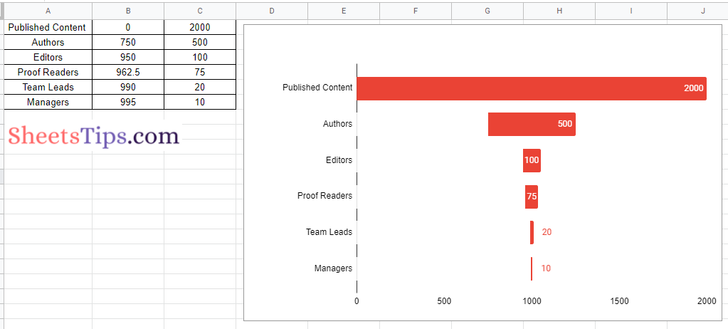
- 7th Step: Now add the “Data Labels” to the Stacked Bar Chart.
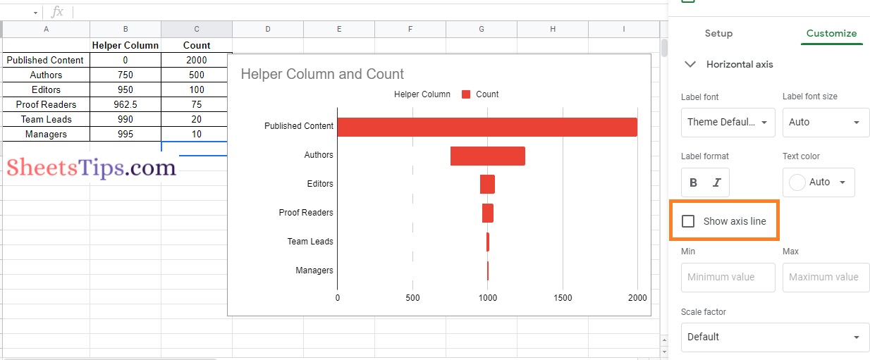
- 8th Step: Finally, remove the x-axis as shown in the image.
Your funnel charts are ready in Google Sheets.
Inserting Funnel Charts using the REPT Function
There are several methods with the help of which we can create funnel charts on Google Sheets. If you do not want to follow the above method, then simply follow the steps listed below to insert the funnel charts into Google Sheets using the REPT function.
- 1st Step: Open the dataset for which you want to create the funnel charts.
- 2nd Step: Move to the cell where you want to generate the funnel chart.
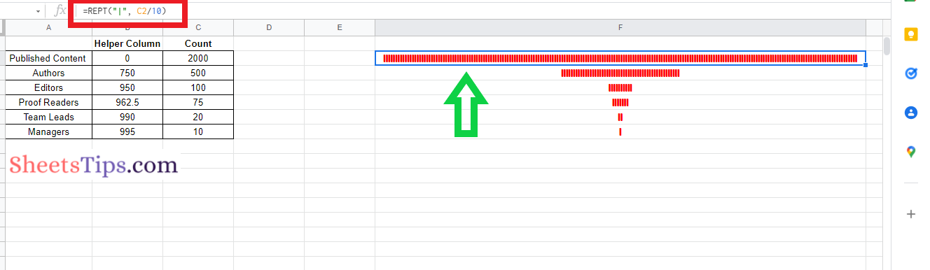
- 3rd Step: Enter the formula as “=rept (“|”B2/10)“.
- 4th Step: Press the “Enter” key and now you will see the results as shown in the image below.
- 5th Step: Using the Fill Handle, drag the columns until the largest bar fits in them.
- 6th Step: Now change the font size to “Modak” and now your results will look like the following image.