
With the help of the Google Sheet IFS Function, we can test multiple conditions and draw the results based on the condition with the same formula. The main difference between the IF function and IFS function is that the IFS function allows us to test multiple conditions at the same time. Whenever the IFS condition is found to be TRUE, the corresponding value is returned.
On this page, we have provided all the necessary information on how to use the IFS function with multiple conditions and important Google Sheet Tips. Read on to find out more.
Table of Contents |
Google Sheet IFS Function Formula
The IFS function syntax which needs to be used in Google Sheet is given below:
=IFS(Condition1, Value1, [Condition2, Value2],…)
- Condition1: This is the first condition that the function examines.
- Value 1: If the first condition is TRUE, Value1 is the value to return.
- [Condition2…Condition127]: You can use up to 127 optional parameters using Condition2 to Condition127. Additional conditions might also be specified here. There must be a value returned in the event that the condition is TRUE for each condition you specify.
- [Value2…Value127]: These are optional arguments. Each value is associated with a condition and is returned if that condition is the first to be TRUE.
Using Excels IFS Function With Example
As discussed above, we can use the IFS function to test multiple conditions. Let’s understand how to use IFS Function in Google Sheets for multiple conditions with examples.
- Using IF Function in Google Sheets: IF Statement Formula & Examples
- How to Extract the Year from Google Sheets-YEAR Function in Google Sheets
- How to Count Cells If Not Blank in Google Sheets
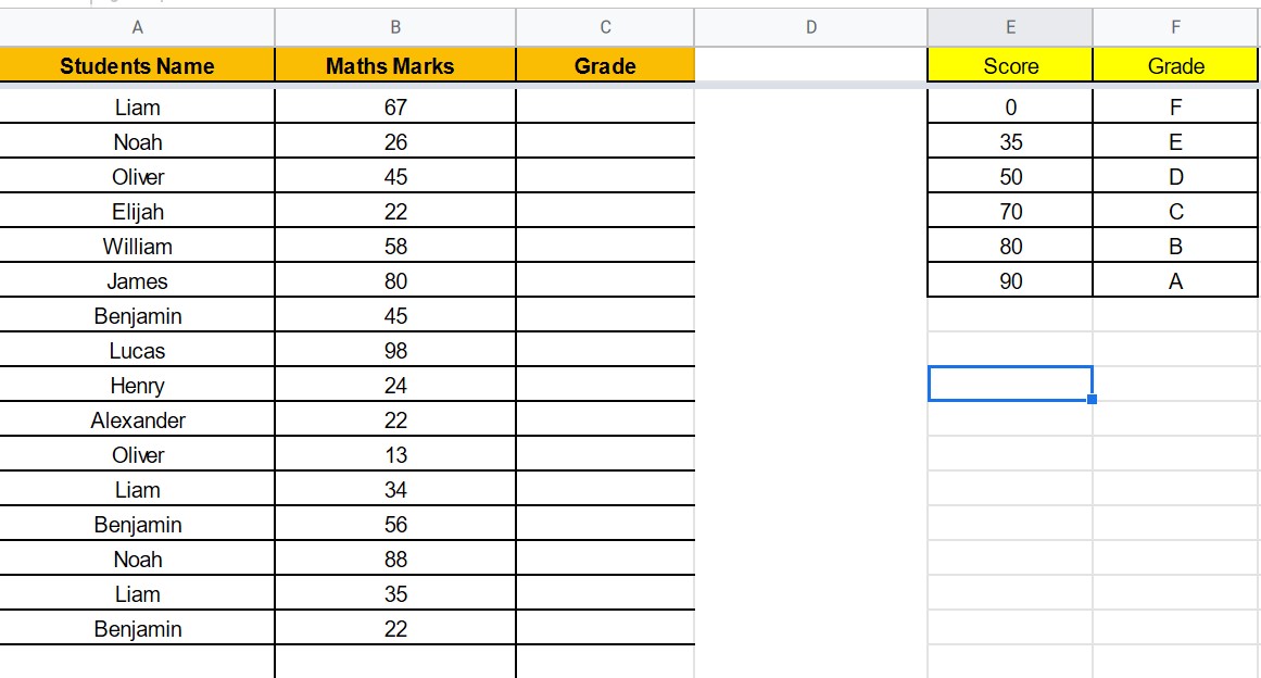
Example 1 – Calculate Student’s Grade From Score Using IFS Function
Let’s understand how to use the IFS function with the help of the following dataset. Now we have students marks and want to map the grades according to the marks scored by the students according to the data entered in Cell “E” and “F“.
Follow the steps listed below to map the student’s grades according to marks with the help of the Google Sheet IFS function.
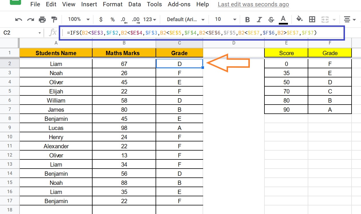
- Step 1: Since I want to map grades in Cell “C“, I am hovering in the “C” cell. Like-wise, you can select the cell where you would like to apply the IFS condition.
- Step 2: Now enter the formula as “=IFS(B2<$E$3,$F$2,B2<$E$4,$F$3,B2<$E$5,$F$4,B2<$E$6,$F$5,B2<$E$7,$F$6,B2>$E$7,$F$7)“
- Step 3: Click on the “Enter” button. Now drag the same formula to all the cells.
You will see the results as shown below.
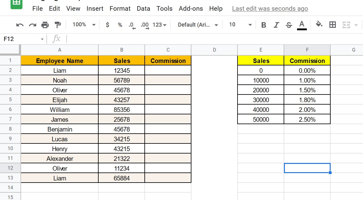
Example 2 – Calculate Commission Based On Sale Value Using IFS Function
Now let’s see how to use the IFS function with another example. In the following dataset, let’s calculate the commission which will be added to the employee salary based on the sales they made as per the data mentioned in Cell “E” and “F”.
Follow the steps listed below to map the commission percentage against the employee name with the help of the IFS function in Google Sheet.
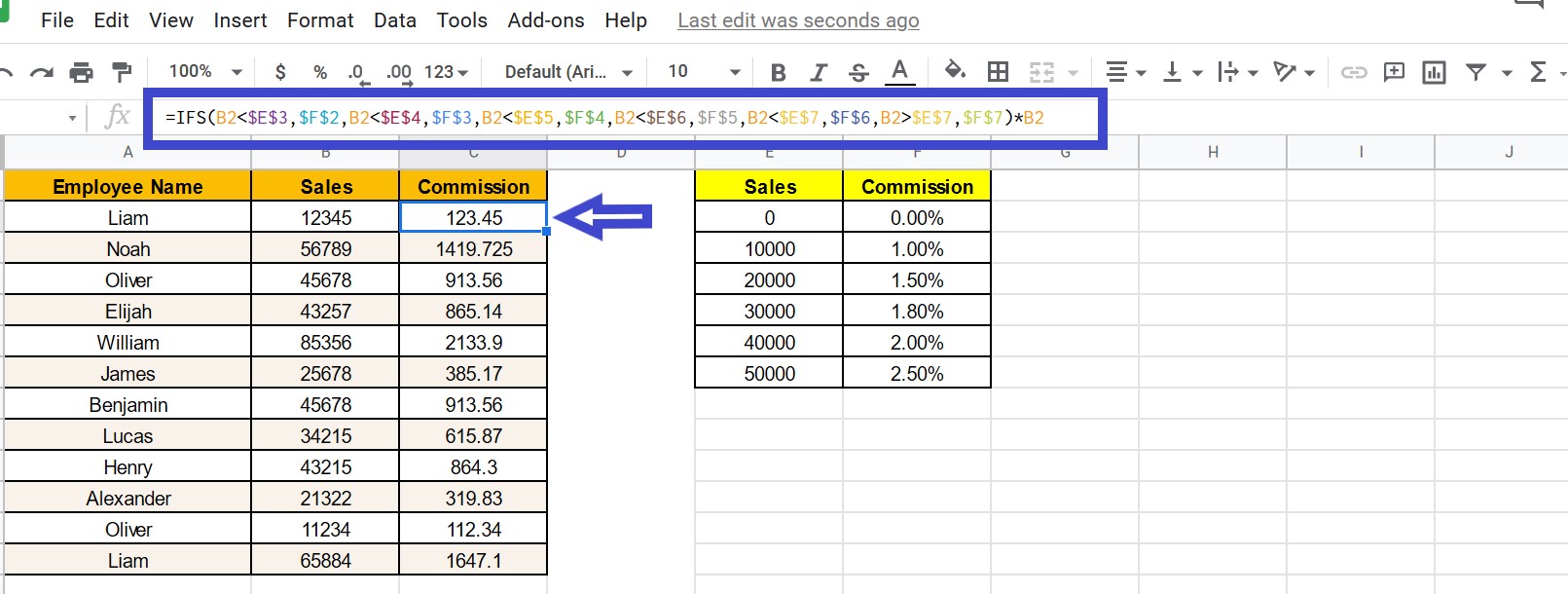
- Step 1: Select the cell where you would like to apply the IFS formula in Google Sheets.
- Step 2: Now type the formula as “=IFS(B2<$E$3,$F$2,B2<$E$4,$F$3,B2<$E$5,$F$4,B2<$E$6,$F$5,B2<$E$7,$F$6,B2>$E$7,$F$7)*B2“.
- Step 3: Click on “Enter”. Now drag the formula to all the cells.
You will see the commission percentage against the employee name as shown below.
Highlights Of IFS Condition In Google Sheets
- The value of the first TRUE condition would be returned by the IFS function. As a result, it’s possible to have many TRUE conditions. However, only the first one’s value would be returned.
- The IFS function must return either TRUE or FALSE for all of its conditions. The formula will return an error if it does not.
- The result of the formula would be a #N/A error, if all of the conditions in the IFS function return FALSE. Because the #N/A error isn’t very useful in determining what happened, set the last Condition to TRUE and the value to FALSE or a descriptive phrase like “No Match.”
IF and IFS Function in Google Sheet
The most significant distinction between the IFS and the IF functions is that the IF function allows you to define what value to return if the condition is FALSE. This feature is not available in the IFS function.
However, when you have several conditions, then the IFS condition would be a great help to get the results.