Google Sheets FACT Function will help the users to find the factorial of a number. Yes, you have heard it right. When you want to find the factorial of a number, you might have to perform mathematical calculations in manual method. However, using the FACT Function in Google Sheets, one can easily find the Factorial of a number.
On this page, let us understand how to use the FACT function in Google Sheets and how to find the factorial of a number using the Sheets Tips provided on this page. Read further to find out more.
| Table of Contents |

FACTORIAL – FACT Function Syntax in Google Sheets
The syntax of the FACT function in Google Sheets is given below:
FACTORIAL Syntax = FACT (value)
Here, the value represents the number (or a reference to a number) for which the factorial will be computed and returned.
If you give FACT a number or a reference to a number containing a decimal portion, the decimal part will be shortened before being calculated.
- Pi Function in Google Sheets: Discover & Generate π Function in Google Sheets
- How to Use SWITCH function in Google Sheets? (With Examples)
- How to Use Google Sheets Weekday Function With Example
How Do You Do Factorials in Google Sheets?
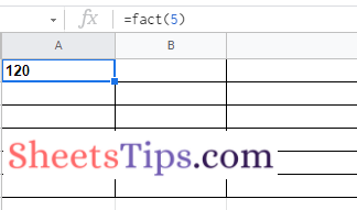
Let us understand how to perform factorials in Google Sheets using an example. Assume that we want to find the factorial of number 5. The steps to get this done in Google Sheets are as follows:
- 1st Step: Launch the Google Spreadsheet on your device.
- 2nd Step: Now move to the cell where you want to find the factorial of number 5.
- 3rd Step: Here enter the formula “=FACT(5)“.
- 4th Step: Press the “Return” key.
- 5th Step: Now you will see the results on the spreadsheet which shows the factorial of number 5.

How To Find Factorials for Array of Numbers in Google Sheets?
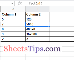
Google Sheets also allows users to find the factorial for an array of numbers. You must simply use the Fill Handle function in Spreadsheet, which helps to find factorials for an array of numbers. The steps to follow to find factorials for the array of numbers in the Spreadsheet are as follows:
- 1st Step: Launch the Google Spreadsheet on your device.
- 2nd Step: Now in Column 1, enter the list of numbers for which you would like to find factorials.
- 3rd Step: In Column 2, against the first number, enter the formula =FACT(A2). {A2 is the cell range}.
- 4th Step: Press the “Enter” button. Now you will see the results.
- 5th Step: Now drag the Fill Handle from the formula applied cells to other cells and now you will see factorials of all the numbers.

How to Find Factorials for Decimal Numbers in Google Sheets?
The Google Sheets FACT function will truncate the decimal part when you try to find the factorial of decimal numbers. Let us understand how to find decimal number factorials in Google Sheets using the steps provided below:
- 1st Step: Open the Google Spreadsheet on your device.
- 2nd Step: Now move to the cell where you want to find the factorial of a decimal number.
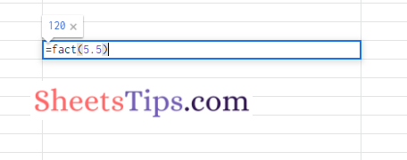
- 3rd Step: Enter the formula “=FACT (5.5)“. I entered 5.5 since I wanted to find the factorial of decimal number 5.5.
- 4th Step: Press the “Enter” key and you will see the factorial of number 5 i.e., 120.

Here, the Google Sheets have truncated the decimal value 0.5 and showed the results for Factorial of number 5.