In Google spreadsheets, combining text and numbers is common. You may need to combine text values with formula results in a range of situations. For example, if you would like to combine text and formula values from 2 different cells into a single cell, then you will have to make use of use of this function. In Google Sheets, merging text with formula involves only the usage of a concatenation operator or function. In this article, let’s understand how to combine formula and text along with important Google Sheet tips. Read on to find more.
Table of Contents |
How to Combine Formula and Text in Google Sheets?
We can combine formula and text in Google Sheets with the help of any of the following two methods:
- Using ampersand (&)
- Using Concatenate Function
Using the Ampersand (&) to Combine Formula and Text
The ampersand sign represents the concatenation operator (&). It’s used to join two or more values together and returns a string with the values attached to each other. As a result, using this operator to merge formula and text into a single cell value is a wonderful method to save time. Let’s say you’ve got the following dataset and want to see the average marks for each row.
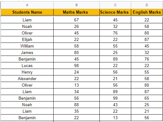
Here is how we can execute it by following the steps as listed below:
- Step 1: Select the first cell where the combined values should display (E2).
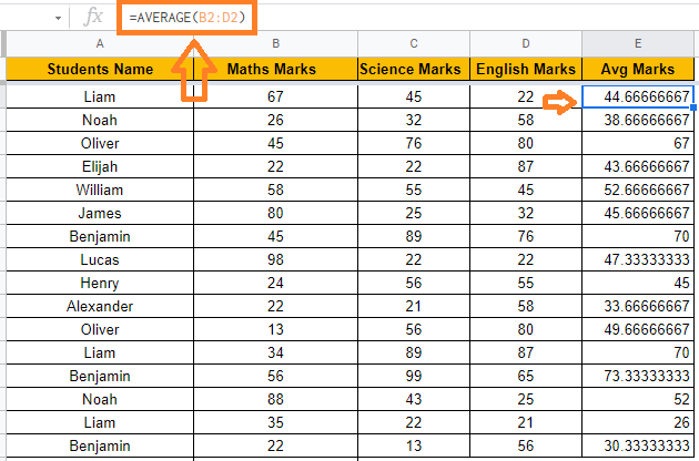
- Step 2: Press the Enter key after typing the formula “=AVERAGE(B2:D2)“.
- Step 3: Cell E2 contains the result of the AVERAGE function. Double-click on the fill handle in the bottom right corner of cell E2 to see the result. This will duplicate the formula to all other cells in column E, giving you separate average marks for each row.
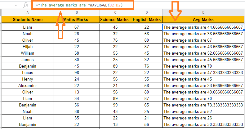
- Step 4: To mix text and formula, type =”The average marks are “&AVERAGE(B2:D2)“. Remember to use double quotes to enclose any string or text value.
- Step 5: Drag the fill handle to the other cells in the E row now. The results will be displayed as follows:
To combine many substrings and values into one, use the concatenation operator. All you have to do is use the ampersand operator (&) to combine each pair of substrings.
- Concatenate in Google Sheets: Concatenate Multiple Cells using Separator, Comma
- How To Insert Indents in Google Sheets? – Know How to Tab Down in Google Sheets
- How to Quickly Merge Cells in Google Sheets: Merge & Unmerge Without Losing Data
Using the CONCATENATE Function to Combine Formula and Text
The CONCATENATE() function is similar to the concatenation operator in terms of functionality (&). The only difference between the two is how they’re used.
The CONCATENATE function has the following general syntax:
=CONCATENATE(text1, [text2],…)
Where text1, text2, and so on are substrings you want to combine.
This function can be used to merge numerous substrings and values into a single value, where each substring is a function parameter.
Let’s put the CONCATENATE function to work on the same dataset as Method 1 by following the steps as listed below:
- Step 1: Select the first cell where the combined values should display (E2).
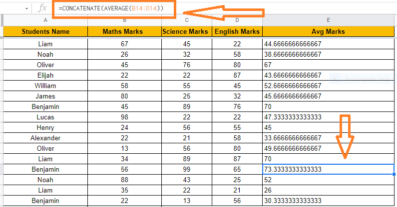
- Step 2: Now type the formula as “=CONCATENATE(AVERAGE (B2:D2 ))“.
- Step 3: Click on the “Enter” button.
- Step 4: In cell E2, you will find the result of the AVERAGE function paired with the text. Double-click the fill handle in cell E2’s bottom right corner. This will duplicate the calculation in all of column E’s other cells, giving you individual AVERAGE marks for each row.
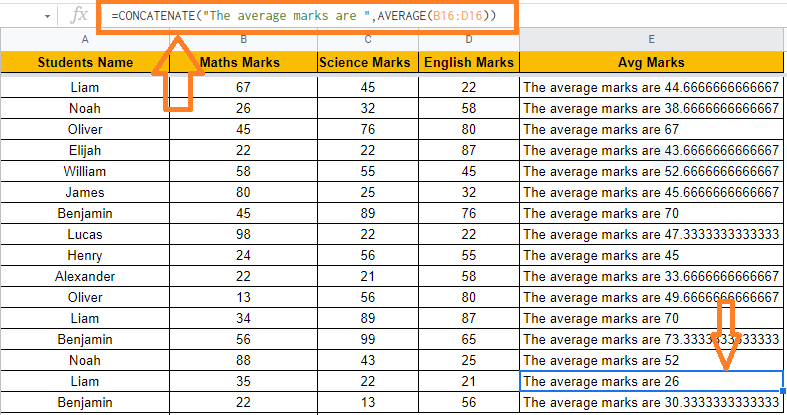
- Step 5: To use the Concatenate function to combine text and formula, type =CONCATENATE(”The average marks are “, AVERAGE(B2:D2)).
- Step 6: You will now be able to see the results. Drag the fill handle to apply the formula to all of the cells. Other cells will show the results as shown below: