When you are doing a data entry task or want to use the same formula for all the cells in Google Sheets, then Fill Handle is for you. The fill handle feature of Google Sheets helps us to save a lot of time and reduces the manual entry of the work.
Consider the case where you need to quickly generate a series of 100 numbers (e.g., 1, 2, 3, etc.). It’s possible to do this manually, but it’s a pointless exercise. Instead, you may get this series in a matter of seconds by using the fill-down feature in Google Sheets. Google Sheets has the ability to autofill numbers based on prior values.
So, let’s understand how to use the Fill Handle with the help of Google Sheets Tips provided on this page. Read on to find out more.
Table of Contents |
What is Fill Handle in Google Sheets?
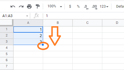
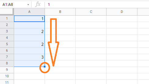
When you choose a cell or a range of cells in Google Sheets, you will see that the selection has a little square on the bottom-right border as highlighted in the image below.
Now let’s understand the Fill Handle Function with the help of examples in the below section of the page.
Filling a Series of Data
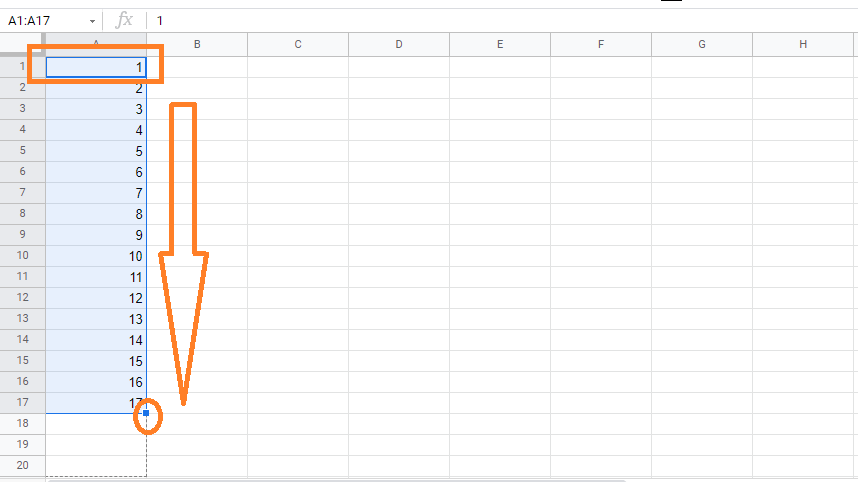
Consider that you want to fill the number series from 1 to 20. Now let’s understand how to do this with the help of the fill handle the feature in Google Sheets.
- Step 1: Open the Google Spreadsheet to use the fill handle feature.
- Step 2: Now move to the row where you would like to start the number series and enter number 1 in Row 1 & number 2 in Row 2.
- Step 3: Then select Row 1 & Row2, here you will see the fill handle feature.
- Step 4: Drag the fill handle till row no 20.
- Step 5: You will see the series of numbers created within a fraction of seconds.
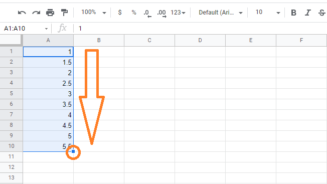
You can also create a series of numbers with the help of decimal points. Suppose, if you want to create a series of numbers such as 1, 1.5, 2, 2.5, and so on, then you can use the fill handle function. The steps which we need to be followed for getting this done are given below:
- Step 1: Go to the row where you would like to create a decimal number series.
- Step 2: Now enter 1 in row 1.
- Step 3: Enter 1.5 in row 2.
- Step 4: Now select both row 1 and row 2 and drag the fill handle.
You will see the decimal number series being created within a fraction of the seconds.
The pointer changes to a + icon when you position it over this small blue square. This means that if you left-click on the mouse or keypad, the fill handle will appear and you may use it to fill down data in Google Sheets.
- How to Sort by Color in Google Sheets: Multiple Color Sort/Filter by Color
- How to Combine Formula and Text in Google Sheets: 2 Easy Methods
- The Ultimate Guide to Using Conditional Formatting in Google Sheets
If you hold down the left mouse key and move the fill handle down, you will find that the cells are automatically filled with various numbers.
The values filled by the fill handle feature will be determined by what you have in the cells that were initially selected or previously selected.
How to Fill Data with Blank Rows?
Consider that you want to create a number series where you have to keep the blank row after every number. So let’s understand how to do this with the help of fill handle in Google Sheets.
- Step 1: Select the row from where you would like to create a number series.
- Step 2: Now enter 1 in Row 1.
- Step 3: Keep Row 2 blank.
- Step 4: Now select both Row 1 & Row 2 and drag the fill handle to see the results.
Fill Month Name & Year in Google Sheets using Fill Handle
The steps to fill the month names in Google Spreadsheets are explained below:
- Step 1: Open the Google Sheets to create a month name using the fill handle.
- Step 2: Now type the name as “January” in Row 1.
- Step 3: Move to Row 2 and enter “February”.
- Step 4: Drag the fill handle by selecting Row 1 & Row 2. You will see the Month name in series order with the help of the fill handle function.
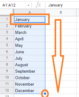
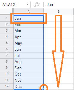
This works because Google recognizes January and February as months. You can do the same thing with month abbreviations like Jan, Feb, and Mar.
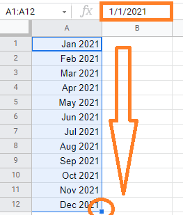
You can also use the year and the month name together. It will be recognized by Google Sheets as a date and will be filled in accordingly.
While month names repeat after all 12 months have been covered, in the case of month names with the year, it will continue on to the months in the following year.
For example, If you want to create a series of months along with a year. So let’s understand how to do this with the help of the steps listed below.
- Step 1: Move to Row 1 and enter Jan 2021.
- Step 2: Then in Row 2 enter Feb 2021.
- Step 3: Now select both Row 1 & Row 2 and drag the fill handle you will see the results.
How to Fill Data Without Dragging the Fill Handle?
We can also fill the data without dragging the cursor. For this select the previous 2 rows and then double click the fill handle “+” icon. You will see the fill handle function filling the data based on the previously selected rows.
Auto Fill-in Google Sheets
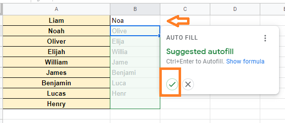
When you are using a formula in Google Sheets, the sheets show the auto-fill feature as soon as you enter the formula in the first cell.
If you click on the Right tick when the suggested autofill feature is shown up, the data will be auto-filled in the Google Sheets.
Alternatively, you can use the keyboard shortcut “Cntrl+Enter” to autofill the sheet.
