Though Google Sheets is a user-friendly spreadsheet software, we tend to experience Formula Parse Errors from time to time. We experience errors for various reasons. This could be a blank cell, a number, or a relevant alert message that we are unfamiliar with. However, we can use the IFERROR function to overcome these errors. The main objective of the IFERROR function is that it helps to clean and remove unwanted error message which is displayed on our Google Sheets.
Also, the IFERROR allows you to “instruct” the spreadsheet as to what value to display if an error is detected. In this article, let’s learn everything about the IFERROR function along with important Google Sheet tips. Read on to find out more.
Table of Contents |
Common Errors That We See in Google Sheets
The common errors that we encounter in Google Sheets are:
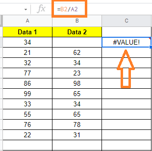
1. #VALUE! Error
It is the most popular type of error in Google Sheets. It happens when you use the wrong data type for the expected input arguments.
2. #REF! Error
This is known as a reference error, and it occurs when the reference in the formula is no longer valid. This could happen if the formula refers to a cell reference that does not exist. For example, if you delete a row/column or worksheet that was referred to in the formula, the Reference error will be shown.

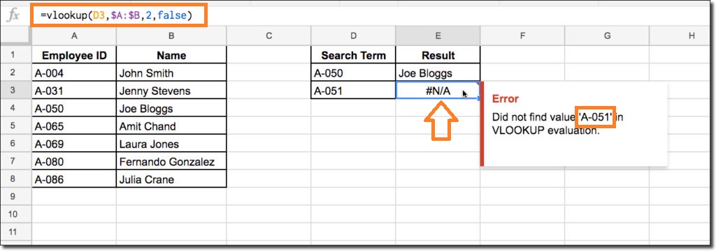
3. #N/A! Error
This is known as the ‘not available’ error, and it appears when you use a lookup formula and it cannot find the value.
4. #NUM! Error
If you try to calculate a very large value in Google Sheets, you may encounter a numeric error. For example, if you are trying to calculate =123^456, it will result in the number or numeric in Google Sheets. It can also happen if you try to enter an invalid number. For example, if you pass a negative number as an argument to the Square Root function, it will return a number error.
- How to Use IMPORTRANGE Function in Google Sheets (with Examples)
- How to VLOOKUP from Another Sheet in Google Sheets: Vlookup Between Two Sheets
- How to Get Running Totals in Google Sheets (Easy Formula)
5. #NAME! Error
This error is most likely caused by a misspelled function. For example, if you use VLOKUP instead of VLOOKUP by mistake, you will get a name error.
Using IFERROR Function in Google Sheets
Let’s understand how to use the IFERROR Function in Google Sheets with the help of examples:
IFERROR Return Blank or Custom Text
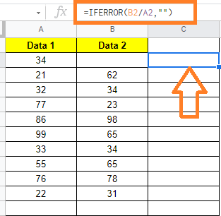
You can easily create conditions that specify a specific value if a formula returns an error. For example, if there is an error then the cell should be blank instead of showing an error.
If you have formula results that are causing errors, you can use the IFERROR function to wrap the formula in it and, in the event of an error, return a blank or meaningful text.
Now let’s understand how to do this with the help of the steps listed below:
- Step 1: Consider the following dataset. Now, we are trying to divide cell A2 divide B2, where B2 is blank. The formula which needs to be entered in Cell C is B2/A2.
- Step 2: Now the cell shows #VALUE! Error.
- Step 3: Now go to the error shown cell and type the formula =IFERROR(B2/A2,””).
- Step 4: The error shown cell is now blank as shown in the image below.
Return ‘Not Found’ instead of #ERROR!
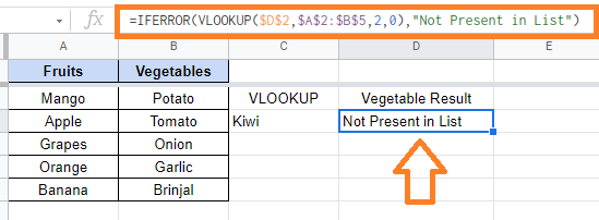
When the VLOOKUP function cannot find the lookup value in the table array, it returns a #N/A! error. instead of the error, you can use the IFERROR function to return meaningful text such as ‘Not Found’ or ‘Not Available’.
Let’s understand how to do this with the help of the steps listed below:
- Step 1: Consider a dataset as shown below. Here we are trying to Lookup Value from the sheet name.
- Step 2: Since the specified data is not available, the VLOOKUP function returns the #ERROR! error.
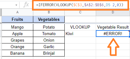
- Step 3: Now go to the cell where #N/A! error is shown. Here enter the formula “=IFERROR(VLOOKUP($D$2,$A$2:$
B$5,2,0), “Not Present in List”)“. - Step 4: Press the “Enter” key.
You will see the error displaying Not Present in List as shown below.