
Google Sheets Named Ranges lets you use a single range across several sheets, formulas, and other operations, and then change it from a specific location. For example, Instead of naming a range of cells “A1:B2,” you may call it “Fruits.” A formula like “=SUM(A1:B2, D4:E6)” could be written as “=SUM(Fruits, Vegetables)” in this way. In this article, let’s understand how to create static and dynamic named ranges with important Google Sheet tips. Read on to find more.
Table of Contents |
How to Create Named Ranges in Google Sheets?
Follow the steps as listed below to create a named range in Google Sheets:
- Step 1: Choose the dataset to create a named range.
- Step 2: From the homepage, select “Data” and then “Named Ranges” from the drop-down menu.
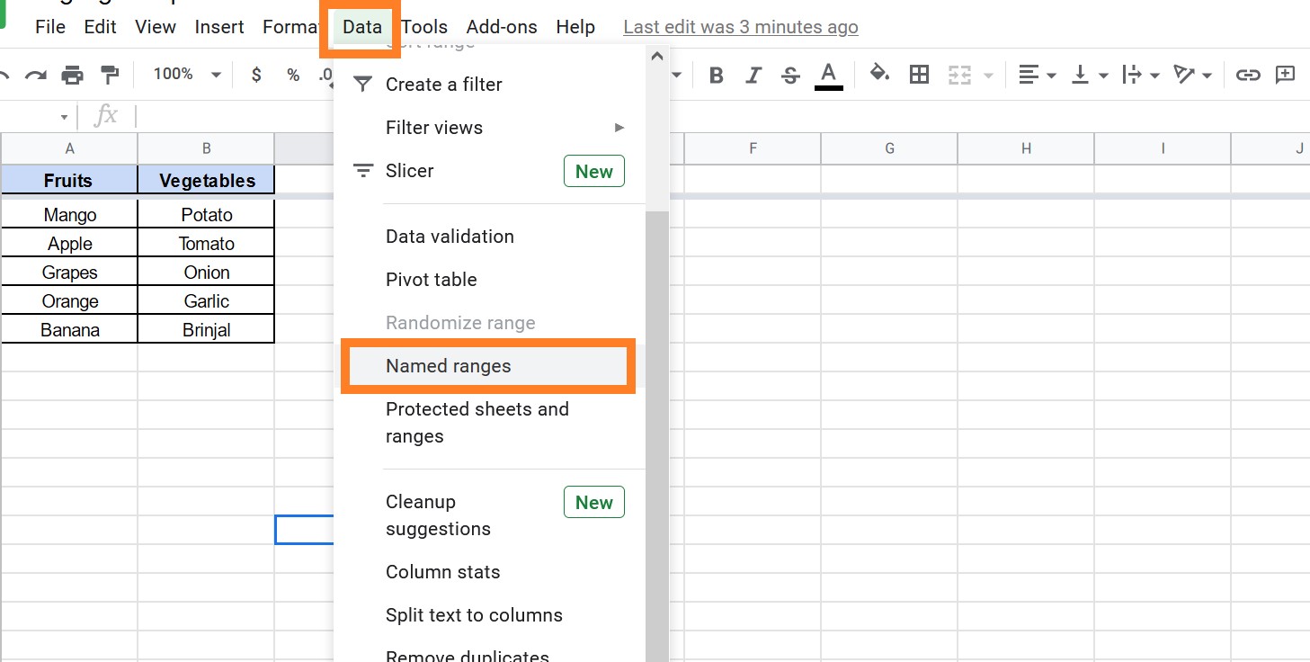
- Step 3: The “Named Ranges” tab in Google Sheets will now open. Now select “Add a range” from the drop-down menu.
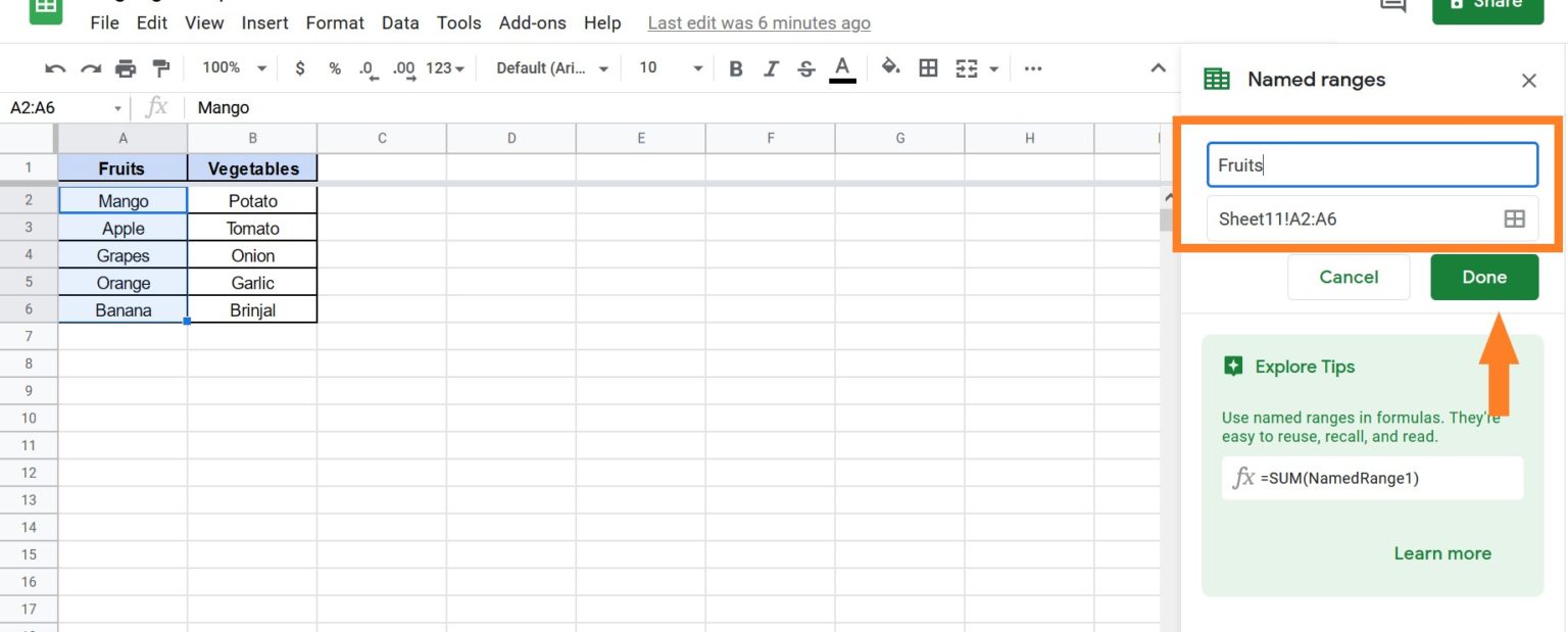
- Step 4: Mention the “Named Ranges” name as well as the cell range.
- Step 5: Select “Done” from the drop-down menu.
List of Rules to be Followed to Create Named Ranges
The list of rules which one should follow while creating a named range is:
- Only letters, numbers, and underscores are permitted.
- Starting with a number or the words “true” or “false” isn’t allowed.
- There are no spaces or punctuation allowed.
- 1–250 characters are required.
- There can’t be any A1 or R1C1 syntax. If you name your range “A1:B2” or “R1C1:R2C2,” for example, you might get an error.
How to Edit Named Ranges in Google Sheets?
We can edit named ranges in Google Sheets by following the steps listed below:
- Step 1: Open the Google Sheet where you would like to edit the named ranges.
- Step 2: Then select Data from the menubar and choose Named Ranges from the drop-down menu.
- Step 3: Click Edit on the identified range you wish to edit or delete.
- Step 4: Enter a new name or range to edit the range, then click the Done button.
- Step 5: To delete the named range, click Delete range next to the name.
- Step 6: Now a pop-up appears. Just click on “Remove“.
Note: Any calculations that reference a named range will no longer operate if you delete it. Protected ranges that refer to a named range will continue to work with the cell values.
- Jump To Cell Range in Google Sheets – How To Jump To Specific Cell Range in Google Sheets?
- How to Extract the Year from Google Sheets-YEAR Function in Google Sheets
- How to Make an Organization Chart in Google Sheets? – Create an Org Chart in Google Sheets
Creating a Dynamic Named Range in Google Sheets
Named Ranges are useful because they allow you to update the named range once and have all the formulas that use it update as well. You may execute this by using a clever INDIRECT function trick. Assume you have a dataset like the one below, and you want to build a named range for the sales data that updates automatically anytime new data is uploaded.
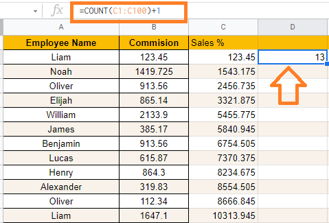
Enter the formula =COUNT(C2:C100)+1 in a cell (D2 in this example). This will tell us how many cells have a number in them. Because our computation data begins in row 2, 1 is added to the formula. It’s also important to note that we use C2:C100 so that any further data will be counted automatically in the future. We also used the COUNT function because the data is purely numerical. COUNTIF can also be used based on your data.
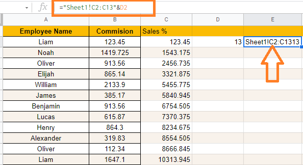
Enter the formula =“Sheet1!C2:C”&D2 in another cell (F2 in this example). This would provide us with a reference for the complete computation data column. For instance, if there are ten sales transactions, Sheet1 will be generated! C2:C11. Sheet1 will be generated if there are 15 transactions! C2:C16.
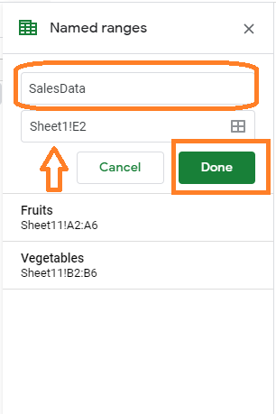
- Select Named Ranges from the Data tab.
- Use Sheet1!E2 as the range name for a named range called SalesData.
You can now refer to the dynamic named range with the following formula: =INDIRECT(SalesData)
The INDIRECT function would refer to cell F2, which has the reference for the sales data, by using the designated range. Because we used =“Sheet1!C2:C”&D2 to make the range in E2 dynamic, the named range also becomes dynamic.
For example, you can now use the formula =SUM(INDIRECT(SalesData)) to determine the total sales. If you add more transaction records, the formula will immediately update and tell you the updated sales total.