Naming a Column in Google Sheets will be very helpful when you are applying formulas. For example, if you have a column name as Employee Salary and when you want to perform some calculations using formulas such as SUM, then you can simply enter the formula as =SUM(Employee Salary) instead of column range such as =SUM(C1) and so on.
On this page, let us understand everything on how to label rows and columns in Spreadsheet using the Google Sheets Tips provided on this page. Read further to find more.

Table of Contents |
How To Name Columns in Google Sheets?
In Google Sheets, we need to use the Named Ranges to name the columns. The named ranges in the Google Sheets will help us to give the cells unique names, ranging from entire columns, rows, or even small groups of cells. The original cell references for example A1, A2, etc. are really not overwritten when you create a named range, but it does make it simpler to refer to these cells and the data contained within them when you are adding new formulas.
- How to SUM a Column in Google Sheets? (Add Numbers, Row, Columns, Cells)
- How to See Basic Calculations Without Formulas in Google Sheets?
- How to Convert Rows to Columns or Backwards in Google Sheets?
Steps to Rename Columns in Google Spreadsheets
Follow the steps as outlined below to rename the rows or columns in the Google Spreadsheet.
- 1st Step: Open the Google Spreadsheet where you want to name the columns.
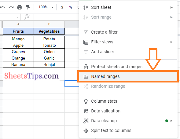
- 2nd Step: Now click on the “Data” tab in the menubar and choose “Named Ranges” from the drop down menu.

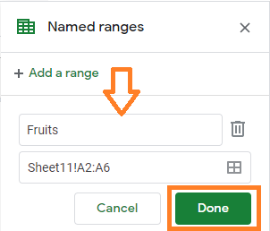
- 3rd Step: The Named Ranges menu will open the spreadsheet towards the right side of the screen.
- 4th Step: Now enter the name of the Sheet in the required box as shown in the image below.
- 5th Step: Then enter the Sheet Range as shown in the cell range box.
- 6th Step: Click on the “Done” button and that’s it. Now the column name has been created for the selected column.

Now instead of using the formula =Len(A1), you can simply use the formula =Len(Fruits) as shown below. This will show the results which are the same as the cell range.

Shortcut to Create Column Name in Google Sheets
The shortcut to name a column in Google Spreadsheets are explained below:
- 1st Step: Open the Google Spreadsheet and select the column to which you want to name.
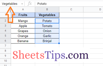
- 2nd Step: Now click on the box which is left towards the formula bar box.
- 3rd Step: Just enter the name of the column.
- 4th Step: That’s it, the column name has been created and you can start performing the calculations using the column name.

By tapping the downward-facing arrow button to the right of the name box, you may see a list of already named ranges. You can pick cells by clicking on any of the named ranges, or you can make changes to existing named ranges by pressing “Manage Named Ranges.”
Keeping Column Headers With Name While Scrolling Down in Google Sheets
We have just created the named ranges for the columns. Now we have to manually enter the column name and set them as headers to make them visible even when scrolling the Sheets. The steps to create the column headers in Google Spreadsheet are explained below:
- 1st Step: Select the column and in the 1st row of the header, enter the name of the column which you want to give.
- 2nd Step: Now click on the “View” tab in the menubar.
- 3rd Step: Choose “Freeze” and now the Freeze sub drop down menu will appear.
- 4th Step: Select “1 Row” from the drop down.

That’s it the rows have been Freezed and now whenever you navigate to the other parts of the sheet, you can see the headers being visible.