VLOOKUP Function in Google Sheets: Finding information across several sheets is one of the most typical issues when working with connected data. Such tasks are common in everyday life, such as scanning wedding plan data for your guest list to determine the invitation status and so on. VLOOKUP in Google Sheets does the same thing: it searches up and pulls matched data from another table on the same sheet or from another sheet.
In this article, let’s understand how to use the VLOOKUP function with important Google Sheet tips.
| Table of Contents |
VLOOKUP Function Syntax
Before performing an operation with the VLOOKUP function in Google Sheets, let’s understand the formula and the parameters of the function.
The VLOOKUP Syntax is:
VLOOKUP(search_key, range, index, [is_sorted])
- search_key – The value to look for in the search key.
- range – The search range to take into account. The key supplied in the search key is searched in the first column of the range.
- index – The value to be returned’s column index, with 1 being the first column in the range. #VALUE! is returned if the index is not between 1 and the number of columns in range.
- is sorted – [TRUE by default] – Indicates whether the searched column (the first column of the provided range) is sorted. In most circumstances, FALSE is the best option.
Example 1: Finding Students Marks Data using VLOOKUP Function
Let’s consider we have the student’s scorecard dataset. Now let’s perform various VLOOKUP Operations in Google Sheets as shown below.
- Step 1: Select the cells where you would like to fetch the values.
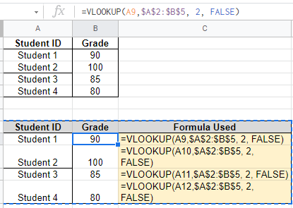
- Step 2: Now type the formula. Here I have used the following formula against the student’s names.
| Student ID | Grade | Formula Used |
| Student 1 | 90 | =VLOOKUP(A9,$A$2:$B$5, 2, FALSE) |
| Student 2 | 100 | =VLOOKUP(A10,$A$2:$B$5, 2, FALSE) |
| Student 3 | 85 | =VLOOKUP(A11,$A$2:$B$5, 2, FALSE) |
| Student 4 | 80 | =VLOOKUP(A12,$A$2:$B$5, 2, FALSE) |
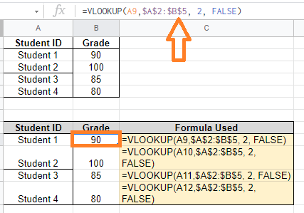
Step 3: Press the “Enter” button to see the results.’
VLOOKUP in the Same Workbook from Another Worksheet
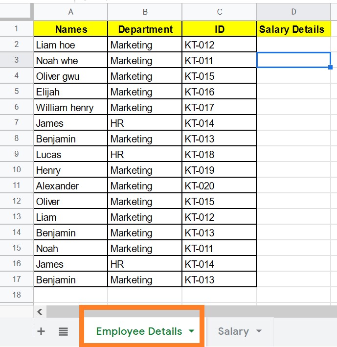
With the help of a basic example, let’s learn how to use the VLOOKUP function. We have two different workbooks in this example: employee details and salary details, as seen below.
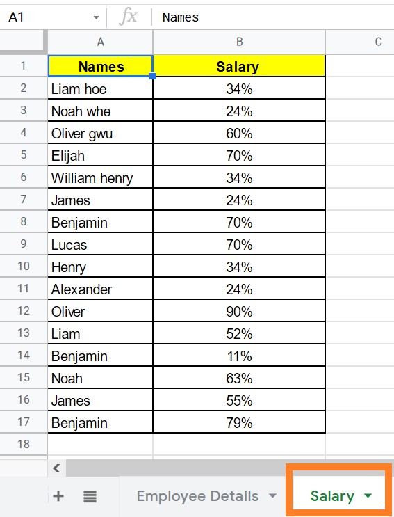
Salary Details
Now we must enter the salary information into the employee information tab. Follow the steps outlined below to call the same.
- Step 1: Choose the cell where the data will be called.
- Step 2: Now type “=Vlookup(A2,Salary!A2:C17,2,false)” into the formula bar.
- Step 3: Press the “Enter” key.
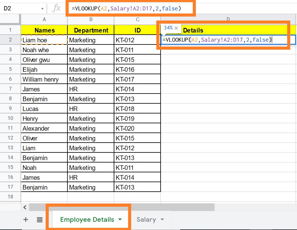
- Step 4: For each cell, drag the same formula.
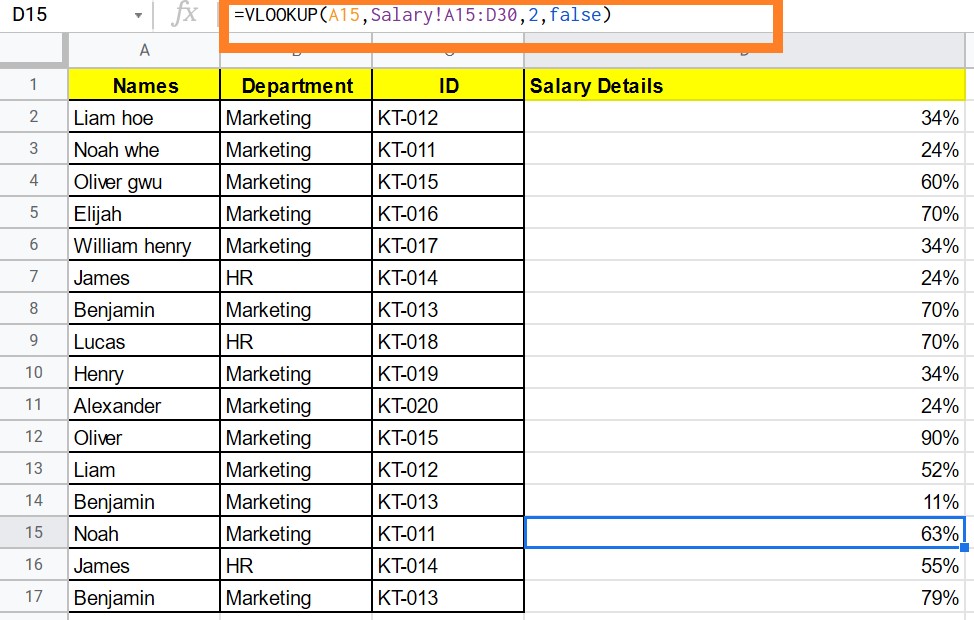
- Step 5: Now you will notice that the Employee Details tab is retrieving salary information.
How does VLOOKUP work for Multiple Matches?
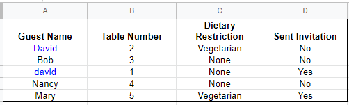
When there are numerous matches for the search key, VLOOKUP returns the first value found. Let’s understand this with the help of the following dataset.
Now we have applied the following VLOOKUP formula as shown in the table below:
| Guest Name | Dietary Restriction | Formula Applied to 2nd Column | |
| david | Vegetarian | =VLOOKUP(A10,$A$2:$C$6, 3, FALSE) | |
| Nancy | None | =VLOOKUP(A11,$A$2:$C$6, 3, FALSE) | |
| Mary | Vegetarian | =VLOOKUP(A12,$A$2:$C$6, 3, FALSE) | |
If you see the above table, we see only the 1st value is returned.