
The wide tables in Google Sheets are pretty common. However, with the help of wide tables in Google Sheets, it is extremely difficult to perform convenient analysis, since we have to keep scrolling the scroll bar horizontally. Also, the wide data in Google Sheets comes handy only when we want to create charts and not for any other purposes. And to overcome these issues, we need to simply convert the wide tables into tall tables which means unpivot the tables in Google Sheets. In order to transpose Google Sheets Pivot Table, we can either use the AppsScript or FLATTEN function.
Let us discuss everything about Google Sheets Flatten Table with the help of Sheets Tips provided on this page. Read further to find more.
Table of Contents |
How To Unpivot a Table in Google Sheets?
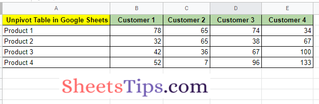
Let us say, we have created a wide table as shown in the image below.
Now we need to convert this wide table into a tall table as shown in the image below.
To transpose the pivot table in Google Sheets, we need to use the flatten function which is discussed in detail in the next section.
- How to Use Slicer in Pivot Tables in Google Sheets (Add/Delete/Customize Slicers)
- Auto Suggested Pivot Chart in Google Sheets: Parameters for Creating Pivot Table Using Explore
- How to Group by Month in Pivot Table in Google Sheets (With Examples)
Reverse Pivot Table in Google Sheets
The steps to reverse a pivot a table in Google Spreadsheet are explained below:
- 1st Step: Open the Google Sheets where you want to unpivot the tables.
- 2nd Step: Now on this page, we are using the table which is shown in the following image as an example. Similarly, create a table that needs to be unpivoted.
- 3rd Step: Move to the cell where you need to unpivot the table in Google Sheets.
- 4th Step: Here we need to combine the data i.e., combine column headings. For this, we need to add special characters between the sections that can be split later. Here I am choosing the special character as “????” smiley to make this more interactive. Choose the special character as per your choice.
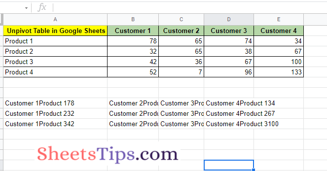
- 5th Step: Simply enter the formula =ArrayFormula(B1:E1&”????”&A2:A4&””&B2:E4).
- 6th Step: Press the “Enter” button and the output result will be as follows.
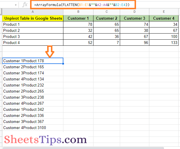
- 7th Step: Now we need to modify this array formula with the help of Flatten function. So our formula will be as follows – =ArrayFormula(FLATTEN(B1:E1&”????”&A2:A4&”????”&B2:E4)).
- 8th Step: Press the “Enter” button and you will see the results as shown below.
- 9th Step: Now we have to use the Split function to split the columns and make it as a tall table.
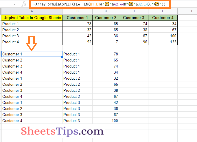
- 10th Step: So our formula will be “=ArrayFormula(SPLIT(FLATTEN(B1:E1&“????”&A2:A4&“????”&B2:E4),“????”)) ” and press the “Enter” button.
Now you will see the wide table is transformed into a tall table as shown in the image below.
We can also unpivot the table in Google Sheets using the Apps Script code.