
We can apply the colour for the specific rows or columns with the help of the Conditional Formatting option available in the menu bar. The data is easier to read when the alternate rows are coloured. These are also called zebra lines.
The Conditional Formatting tool in Google Sheets allows you to format cells based on certain criteria, such as whether they contain a specific word or number.
Also Read: Python Program to Find Sum of Odd Numbers Using Recursion in a List/Array
In this article, let us understand how to add colourful stripes in google sheets with the help of Google Sheet tips. Read further to find more.
Table of Contents |
How to Colour Alternative Rows in Google Sheets?
We can colour alternative rows in google sheets with the help of the Conditional formatting tool. Below are the steps to colour alternative rows in google sheets,
- Step-1: Select the cells in which you want to colour the rows
- Step-2: Click on the Format tab and select the Conditional Formatting option from the toolbar
- Step-3: Scroll down in the Format Rules box and Select ‘Custom Formula is‘ from the ‘Format cells if’
- Step-4: Enter the formula =ISEVEN(ROW()) in the below field.
- Step-5: Choose a formatting style to apply specific colours. You can either choose the default selection or use the toolbar below it to access other Fill colour possibilities.
- Step-6: Click on Done to view the changes you have made.
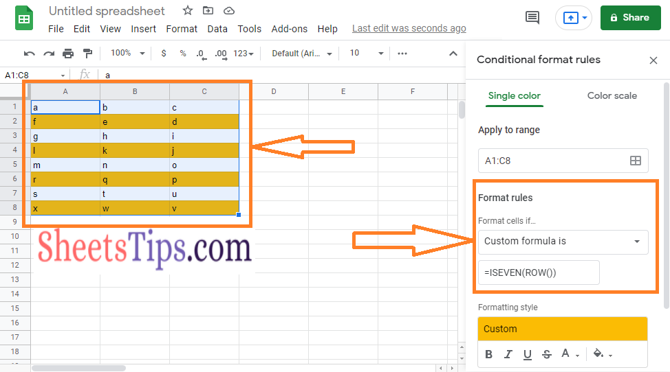
In the above formula – =ISEVEN(ROW()),
It returns true for all cells with an even row number. This formula is checked in each cell through conditional formatting, and every cell that returns TRUE is filled with the given colour.
- How to Color Alternate Rows in Google Sheets: Alternating Colors Every 2 Rows, 3 Rows
- How To Highlight Duplicates In Google Sheets?
- How to Remove Zero Value from Google Spreadsheet? (3 Easy Methods)
In order to colour the odd rows, then you could use formula – =ISODD(ROW())
How to Colour Alternative Columns in Google Sheets?
We can colour alternative columns in google sheets with the help of the Conditional formatting tool. Below are the steps to colour alternative columns in google sheets,
- Step-1: Select the cells in which you want to colour the columns.
- Step-2: Click on the Format and select the Conditional Formatting option from the toolbar
- Step-3: Scroll down in the Format Rules box and Select ‘Custom Formula is‘ from the ‘Format cells if‘
- Step-4: Enter the formula =ISEVEN(COLUMN()) in the below field.
- Step-5: Choose a formatting style to apply specific colours. You can either choose the default selection or use the toolbar below it to access other Fill colour possibilities.
- Step-6: Click on Done to view the changes you have made.
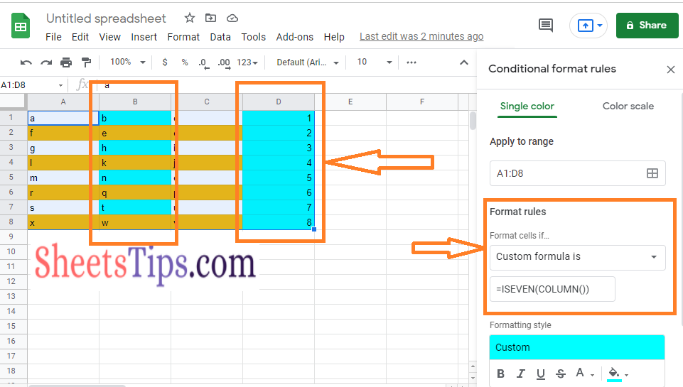
In the above formula – =ISEVEN(COLUMN()),
It returns true for all cells with an even column number. This formula is checked in each cell through conditional formatting, and every cell that returns TRUE is filled with the given colour.
In order to colour the odd column, then you could use formula – =ISODD(COLUMN())
How to Colour Every Third in Google Sheets?
Let us understand how to colour every third row or column with the formula below,
- For colouring every third row, use the formula =MOD(ROW(),3)=0
- For colouring every third column, use the formula =MOD(COLUMN(),3)=0
Below are the steps to colour every third row,
- Step-1: Select the cells in which you want to colour the rows
- Step-2: Click on the Format and select the Conditional Formatting option from the toolbar
- Step-3: Scroll down in the Format Rules box and Select ‘Custom Formula is’ from the ‘Format cells if’
- Step-4: Enter the formula =MOD(ROW(),3)=0 in the below field.
- Step-5: Choose a formatting style to apply specific colours. You can either choose the default selection or use the toolbar below it to access other Fill colour possibilities.
- Step-6: Click on Done to view the changes you have made.
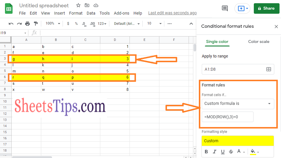
The formula =MOD(ROW(),3)=0 returns TRUE for all cells that return 0 as the remainder, and that cell is highlighted with the given colour.
You may use the same logic to every fourth, fifth, sixth, and so on row.
Similarly, you can use the formula =MOD(COLUMN(),3)=0 for colouring every third column in google sheets.