
The Google Spreadsheet usually doesn’t format numbers by default. So when you are working with Google Sheets to perform basic calculations with numbers such as budget analysis or accounting, then it would be extremely difficult to read the numbers. This is where we want to customize the number format in Google Sheets as per our needs to make it more readable. And thankfully, Google Sheets allows us to create custom number formats as per our needs. In this article, we will learn everything about how to create or customize the number format using the Google Sheets Tips. Read further to find more.
Table of Contents |
How to Change Number Format in Google Sheets?
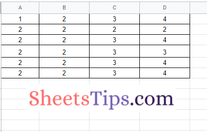
Consider the following dataset. Here the entered numbers are looking normal.
- How to Change Currency Symbol in Google Sheets? (Set Custom Currency Symbol)
- How to Create Candlestick Chart in Google Sheets (With Examples)
- How to Make Tables in Google Sheets? Using Google Sheets Formatting Options
Now the steps to change the number format in Google Spreadsheet are explained below:
- 1st Step: Open the Google Spreadsheet on your device where you want to change the number format.
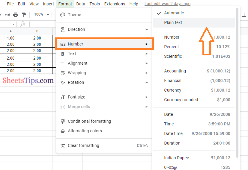
- 2nd Step: Now on the homepage, click on the “Format” tab.
- 3rd Step: From the Format tab drop down, choose “Number”.
- 4th Step: Now the Number sub menu drop down will open on the screen. Here various formats of numbers will open on the screen such as Number, Percentage, Scientific, Accounting, Financial, Currency, and Currency Rounded.
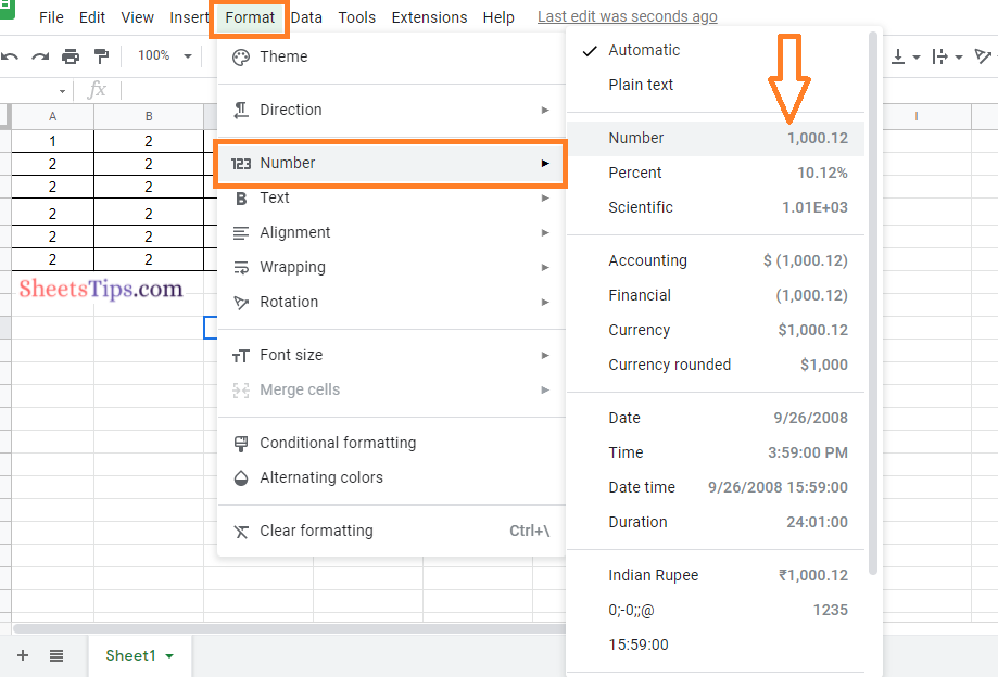
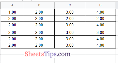
- 5th Step: Choose the required number format. For example, here we are going to choose only Numbers from the option and now the number formats have been changed in the Google Sheets.
How To Create Custom Number Format in Google Sheets?
Google Sheets also allows the user to create a custom number format as per our requirements. Let say that you want to display a number with the Dollar sign without using decimal points but want to include the commas in between; which is a customized number format. We can achieve this using the steps given below:
- 1st Step: Open the Google Spreadsheet on your device.
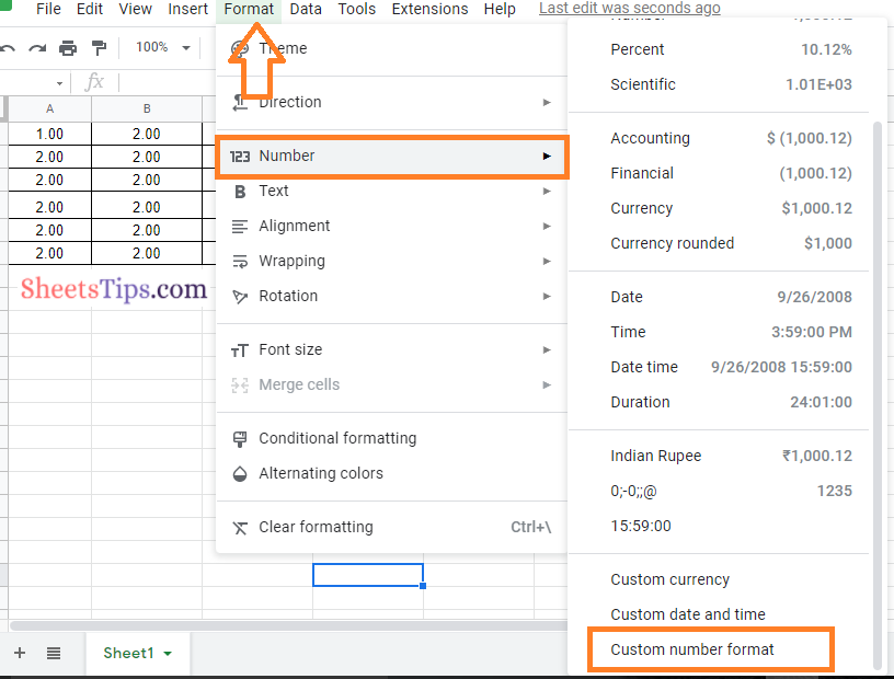
- 2nd Step: Now on the homepage, select the cell range where you need to customize your numbers and then click on the “Format” tab in the menubar.
- 3rd Step: Choose “Number” from the drop-down menu. Now the Number sub drop down menu will open on the screen.
- 4th Step: Scroll to the end of the Number sub drop down menu and click on “More Formats“.
- 5th Step: From the More Formats drop down list, select “Custom Number Format“.
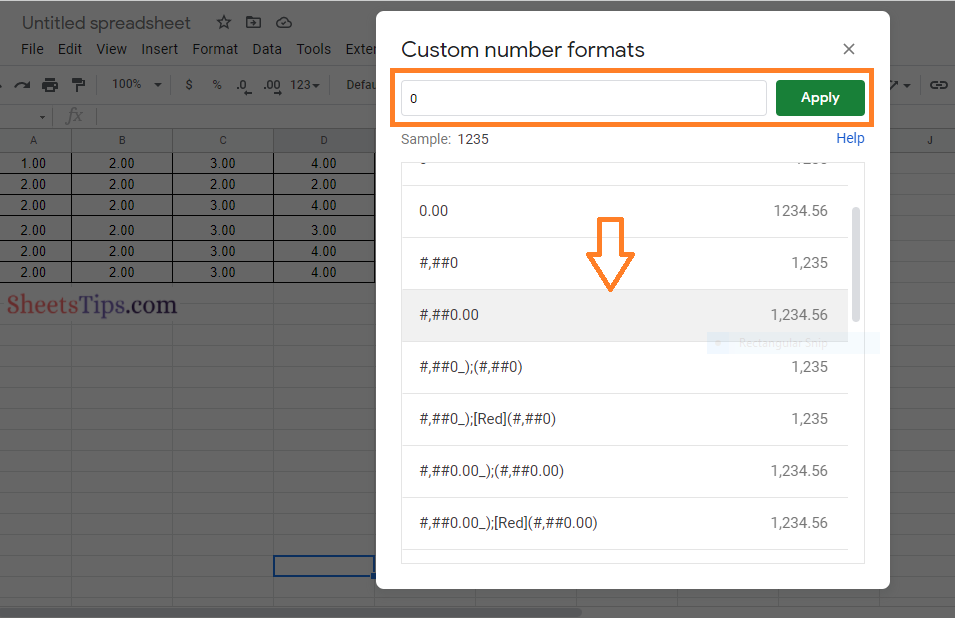
- 6th Step: Now the “Custom Number Formats” window will open on the screen. Scroll down to discover all of the number formats that have been produced for you. The list is separated into two columns as you can see. The number format is shown in the right column, and the syntax for displaying it is shown in the left column.
- 7th Step: Customize the number as per your requirements in the Custom Number Format box. To get this done, the Hash (#) symbol is the only syntax you will need to know. It serves as a substitute for a digit. Everything else remains the same (such as decimal points, dollar signs, and zeros).
- 8th Step: Now For example, if you wish to format a long number as “$1,00,000,” use the “$#,##0.00” syntax. If you don’t want to include the decimal points, just type “$#,##” in that custom number format field.
- 9th Step: Click on the “Apply” button.
These steps will customize the numbers as per your choice.
How to Remove Number Format in Google Sheets?
Once we are done with our work, we might fall under the situation where we need to remove the number format in Google Sheets. The steps to remove the number format in Google Spreadsheet are explained below:
- 1st Step: Open the Google Spreadsheet on your device from which you want to remove the numbering format.
- 2nd Step: Select the range of cells for which you want to remove the number format.
- 3rd Step: Now on the homepage, click on the “Format” tab and choose the “Number” option from the drop down menu.
- 4th Step: Here the “Number” sub drop down menu will open on the screen. Now choose “Plain Text“.
That’s it, the number format which you have applied for the cells has been removed.