When you are working with a huge dataset, then it is extremely difficult to understand which cells are blank and which cells are showing errors. Thanks to the Google Sheets Conditional Formatting feature which helps the Google Sheets user to highlight the blank cells or the cells with errors. However to highlight blanks and error cells one must enable some formatting rules in Conditional Formatting which we will discuss on this page. On this page, let us understand everything on how to highlight blank cells or cells with errors using the Google Sheets Tips. Read further to find more.
Table of Contents |
How to Highlight Blank Cells in Google Sheets?
Follow the steps as outlined below to highlight the blank cells in Google Spreadsheet:
- 1st Step: Open the Google Spreadsheet where you want to highlight the blank cells.
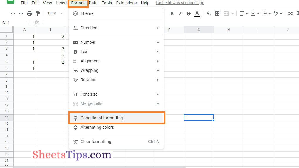
- 2nd Step: Now on the homepage, click on the “Format” tab in the menu bar.
- 3rd Step: Choose “Conditional Formatting” from the drop down menu.
- 4th Step: This opens the Conditional Formatting pane towards the right side of the screen.
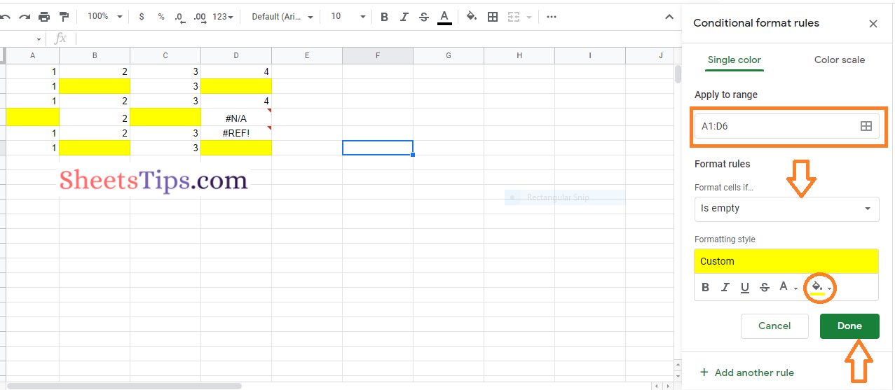
- 5th Step: Now under the “Format Rules” pane, click on the “Format Cells If” drop down menu.
- 6th Step: From the drop down menu, choose “Is Empty”.
- 7th Step: Now come to the Formatting Style section and click on the “Fill Color” icon.
- 8th Step: From the standard color pane, choose the color in which you want to highlight the blank cells. Alternatively, you can customize the color in which you would like to highlight the blank cells using Hex color code under the Custom section in the Fill Color pane.
- 9th Step: Click on the “Done” button and that’s it, you will see the empty cells being highlighted.
- How to Search in Google Sheets and Highlight Matching Data? (4 Easy Methods)
- How to Use Paste Special Options in Google Spreadsheet? Google Sheets Paste Special Explained
- The Ultimate Guide to Using Conditional Formatting in Google Sheets
How to Highlight Errors in Google Sheets?
Now we learned how to highlight the empty cells in the Google Sheets. In some instances, we might also need to highlight the cells with errors along with the empty cells. To get this done, we need to make use of conditional formatting. The steps to highlight errors in the spreadsheet are explained below:
- 1st Step: Launch the Google Spreadsheet in which you want to highlight the cells with errors.
- 2nd Step: Click on the “Format” tab from the menu bar and choose “Conditional Formatting” from the drop down menu.
- 3rd Step: Now move to the conditional formatting pane which is displayed towards the right side of the screen.
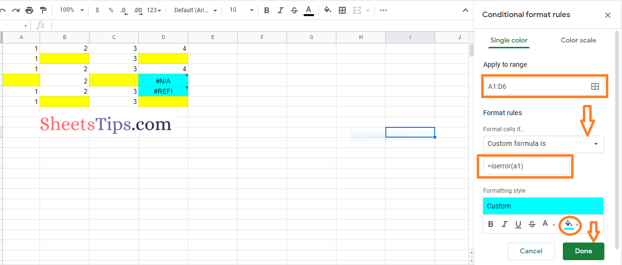
- 4th Step: Under Apply to Range, choose the cell range where you want to highlight the errors.
- 5th Step: Move the cursor to Format rules and hit the “Format Cells if” drop down menu.
- 6th Step: From the drop down menu, choose “Custom Formula is”.
- 7th Step: Now under the Value or Formula section, enter the formula =iserror(cell range).
- 8th Step: In the “Formatting Style”, click on the “Fill Color” option.
- 9th Step: The fill color pane will open. If you want to use Google Sheets default colors, you can choose the standard colors from the Fill Color Pane. Else click on the “Custom” section and customize the colors to highlight the cells with errors.
- 10th Step: Click on the “Done” button and the error cells will be highlighted with the color chosen.