
When you are working with Google Sheets which needs to be shared with multiple users, you might fall under a situation where you might want to hide columns from certain users which is impossible. However, there are few hacks with the help of which you can hide the columns in Google Sheets from certain users. In this article, let us understand how to hide columns/rows from certain users with the help of Google Sheet hacks provided on this page. Read on to find more.
Table of Contents |
Hiding Columns in Google Sheets
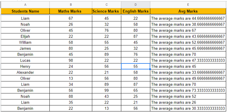
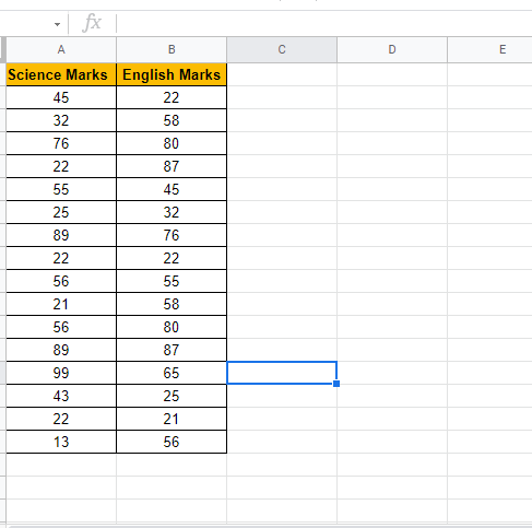
Consider the following dataset where you want to hide columns B and C.
We can easily hide the columns in Google Sheets with the help of the steps provided below:
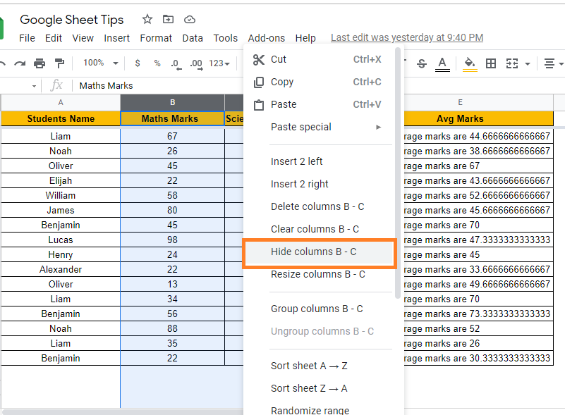
- Step 1: Select the column headers which you would like to hide.
- Step 2: Now Right-click anywhere on the screen.
- Step 3: The context menu will open. Now select “Hide Column” from the drop-down menu.
- Step 4: The selected columns will be hidden now as shown below.
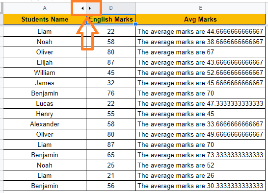
Note: This method is used to hide columns temporarily. If any user clicks on the hidden arrow, then the hidden columns will be unhidden. However, if you use this method while printing the worksheet, the hidden columns will not be printed.
Know how to Unhide Columns.
Since this is a temporary hiding method of columns, let’s use a protected range method to hide columns from certain users in Google Sheets.
- How to Group Columns in Google Sheets? (Group Multiple Columns, Collapse)
- How to Split Text to Columns in Google Sheets: Split Cell Horizontally/Vertically
- How to Create Filter Views in Google Sheets? (Share/Delete/Save/Duplicate Filter Views)
Use Protect Range Feature to Hide Columns from Certain Users
With the help of Protect Range feature in Google Sheets, we can restrict certain users to edit the selected range of cells, be it column or row. Let’s understand how to hide columns with the help of the Protected range feature in Google Sheets by following the steps listed below:
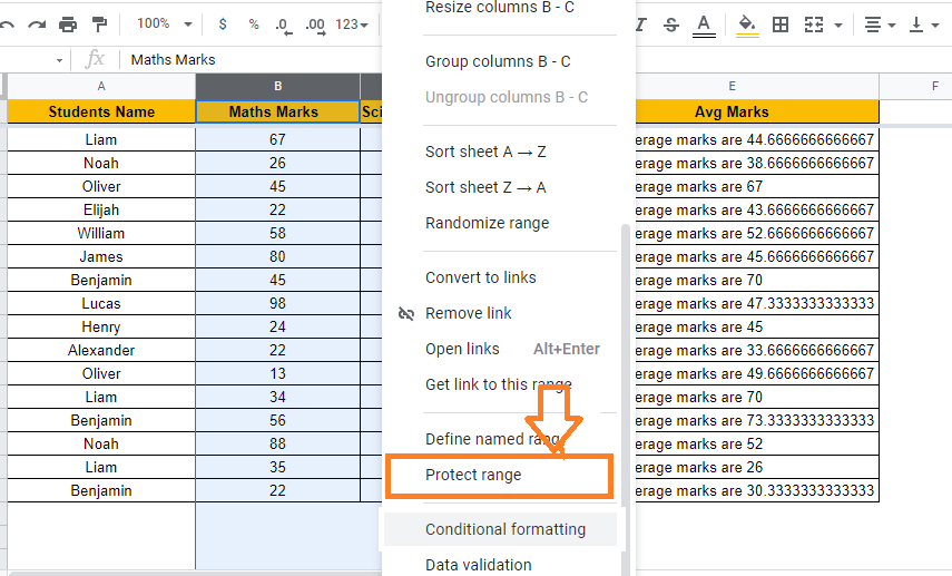
- Step 1: Select the headers of the columns which you would like to hide and Right-click anywhere on the sheet.
- Step 2: Now the context menu will open on the screen. Here select “Protect Range” from the drop-down menu.
- Step 3: Protect Sheet and ranges sidebar will open on the screen. Now enter the cell range in the Range window.
- Step 4: Now click on the “Set Permissions” button.
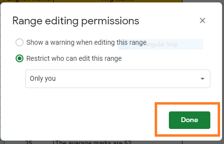
- Step 5: Now the Range Editing Permission window will open on the screen. Now check the “Restrict who can edit this range” box.
- Step 6: Under “Choose who can edit” you will be provided with the list of users who have edit access to the sheet. You can simply uncheck their email ids. Doing so will protect the selected columns by shared users.
- Step 7: Click the “Done” button.
- Step 8: Now again move to the column headers and right-click anywhere on the cell.
- Step 9: Select “Hide Columns” from the context menu and this will hide the selected columns.
Note: You will see that the columns have been hidden, but users who don’t have edit access will not be able to unhide them, so they won’t be able to see them or make any edits.
Nevertheless, there’s a snag in the works: There is still a chance that they will be able to see the content of this column. This is because, if the shared persons make a copy of this sheet, then they can easily see the unhidden columns and make changes in the copy sheet.
Using IMPORTRANGE Function to Hide Columns from Certain Users
IMPORTRANGE Function in Google Sheets helps us to access data from one workbook to another sheet. Thus we can use the IMPORTRANGE function to hide columns from certain users in Google Sheets. Let us understand how to do this with the help of the steps given below:
- Step 1: Firstly, create a private Google Sheet which contains the columns that need to be hidden from certain users.
- Step 2: Now share this private Google Sheet to the selected users to whom you wish to make the columns accessible.
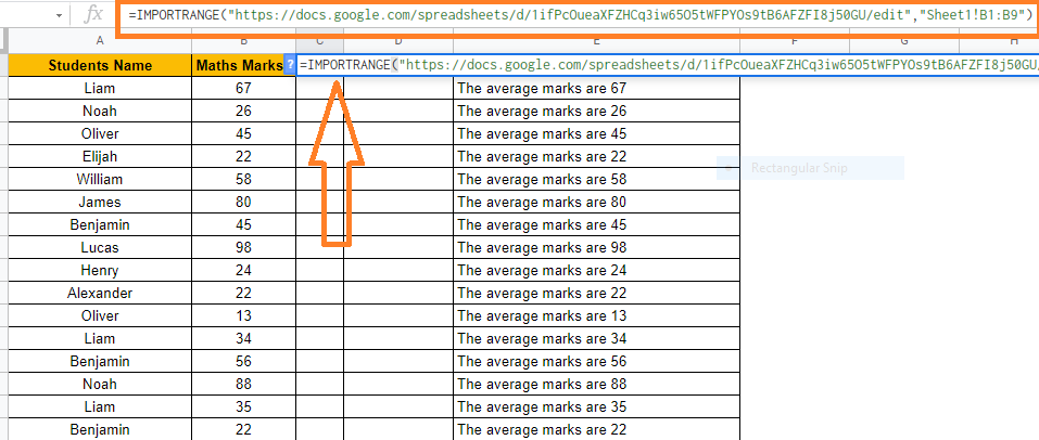
- Step 3: Then move to the Sheet which is been shared with others. Here go the column and use the IMPORTRANGE function to import the columns.
- Step 4: The formula to IMPORT the columns in our case is “=IMPORTRANGE(“url”,”Sheet1!B1:B9)“.
- Step 5: Press the “Enter” button.
- Step 6: Now the columns will be imported. Then protect the columns with the help of steps provided in the previous section.
- Step 7: Then Right-click the columns which need to be hidden and select “Hide Column” from the context menu.
- Step 8: Now the columns will be hidden.
How does this work?
In this case, all of the columns will be copied to the new sheet once more. The user can still see that there are some columns that are hidden.
When they try to unhide the columns, they will encounter a #REF! error. They will see a message that says, “You don’t have permission to access that sheet,” when they hover over the cell containing the error message.
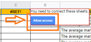
This is due to the IMPORTRANGE function attempting to access a file to which the user does not have access. If you want to make changes to the data in the hidden columns, you must do so in the private file. Because the IMPORTRANGE function is dynamic, any changes you make will be automatically reflected in your shared file.