
Compound Interest in Google Sheets: Almost all of us have learned about compound interest in maths when we were at our schools and colleges. It is one of the most important concepts for banking and finance. Compound interest, basically, is the interest generated for a particular span of time depending upon the principal capital and interest generated in the past periods.
In this article, we will elaborate on this topic more to get your concepts crystal clear and also teach you how to calculate compound interest on a monthly, annual, or daily basis. We will also talk about the various financial formulas as well as growth parameters in these amazing Google Sheet Tips.
- Google Sheets Compound Interest Formula
- How to use the Compound Interest formula in Google Sheets?
- Annual Compound Interest formula in Google Sheets
- Google Sheets Monthly Compound Interest
- Daily Compound Interest in Google Sheets
- Google Sheets Compound growth formula
- Google Finance Sheets formulas
- Google Sheets Investment Calculator
- FAQs
Google Sheets Compound Interest Formula
Let’s understand how to compute compound interest with a proper formula. The following compound interest formula will help you find the ending value of some investment after a certain period of time: A = P(1 + r/n)nt , where:
- A: Final total Amount
- P: Initial Principal Capital
- r: Annual Rate of Interest
- n: Number of compounding periods per year
- t: Number of years
Let us consider a principal capital P, levied with an interest rate of R. At the end of the first year, the total amount will be P+(P*R), or P(1+R) and for the second year, it is going to be P(1+R)+P(1+R)*R, or simply P(1+R)2. Similarly, for the third year, the amount standing will be P(1+R)2+P(1+R)2*R, or P(1+R)3. So, if we consider N as the number of years, the formula for compound interest will be: Compound Interest= P(1+R/t)(n*t), or P(1+R)N.
How To Use the Compound Interest Formula in Google Sheets?
The above formula can be easily applied in Google Sheets to compute the compound interest for a specific span of time. There are two ways in which we can do this:
- Using the general compound interest formula,
- Using the Google Sheets FV Function
Let us now look at how we can apply each of these methods to compute the compound interest for monthly, annual, and daily cases in further sections of this article.
Annual Compound Interest Formula in Google Sheets
To understand this, let’s say you have an initial investment of Rs 2,000 and want to know the future value (or compound interest) after adding a 5% rate of interest on it annually. First, let’s write the initially given parameters in a Google Sheets compound interest template like the below: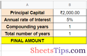
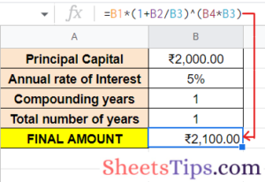
- Using the general Google Sheets Compound Interest Formula: The first way to find the compound interest is to apply the same general Google Sheets Compound Interest formula as mentioned in the previous section. The syntax of the formula is as follows: =B1*(1+B2/B3)^(B4*B3)
Apply this formula to the result in cell B6 of the compound interest spreadsheet, and here’s the result you get for one year:
To find the total amount in 5 years, just replace the value in cell B4 with 5, and the resultant amount would be as follows: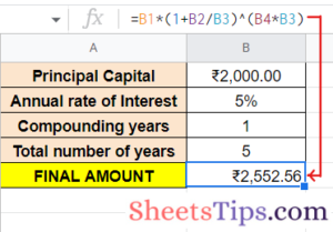
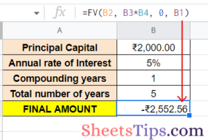
- Using the Google Sheets FV Function: The second way to compute this compound interest is by using the FV function, which is basically used to find out the future value of your investment for a certain period of time at a fixed interest rate.
The syntax for the function is: =FV( rate, number_of_periods, payment_amount, [ present_value], [ end_or_beginning ]), where:
- rate is the rate of interest during the period.
- number_of_periods is the years for which you want to calculate the future value.
- payment_amount is the additional payment made during each period.
- present_value is the principal capital amount. This value is optional.
- end_or_beginning is the integer value that specifies when the payment is due.
Let’s use this FV formula in the following example to calculate the compound interest: =FV(B2, B3*B4, 0, B1). The result is as follows:
Google Sheets Monthly Compound Interest
Now, let’s take another case where 5% is compounded monthly instead of once a year. As mentioned earlier, write the given parameters and then apply the required formulas.
- Using the general Google Sheets compound interest formula, in this scenario, we need to first change the number of periods in a year into months. Since interest is compounded monthly, the number of periods in a year will be 12. Now let’s insert this value into our original compound interest formula.

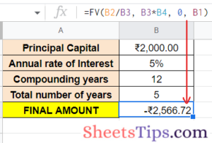
So, at the end of 5 years, the total amount will sum up to Rs 2566.72 when a 5% rate of interest is compounded on a monthly basis.
- Using the Google Sheets FV Function: The FV function for this problem will change a little bit from the previous one. The interest is compounded 12 times in a year for 12 months, so your rate of interest per month will become rate/12, and the number_of_periods is the number of periods in a year multiplied by the number of years.
- rate= B2/B3
- number_of_periods= B3*B4
- payment_amount= 0
- present_value= B1
- end_or_beginning= 0 (by default)
Daily Compound Interest in Google Sheets
Finally, let us consider the last case in which the interest of 6% is compounded daily for 5 years. Let’s see the steps to find the compound interest for the same:
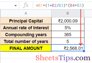
- Using the general compound interest formula, since the interest will be compounded daily, the number of periods in a year will be 365. Now, let’s insert this value into our original compound interest formula. So, at the end of 5 years, the total amount will be Rs 2568.01 when a 5% rate of interest is compounded on a daily basis.
- Using the Google Sheets FV Function- The interest is compounded 365 times in a year, so your rate of interest per day is going to be rate/365, and the number_of_periods is 365 multiplied by the number of years. Replace the value in cell B3 which is the compounding periods per year with 365 and put the formula: =FV(B2/B3, B3*B4, 0, B1). Here is the future value for the given investment at the end of 5 years after being compounded daily:
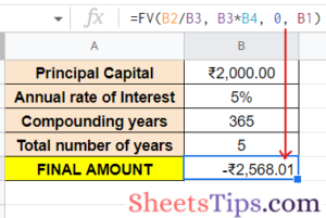
When we specify the present_value (or Principal amount) as a negative number the returned result will be a positive number while giving the FV function.
Google Sheets Compound Growth Formula
CAGR or Compound Annual Growth Rate is used in your spreadsheets to calculate the productive growth rates but is not a built-in formula in Google Sheets, so you will need to do the computation yourself. The syntax for the CAGR formula is =EV / BV ^ (1/n) – 1, where:
- EV and BV are the ending and beginning values.
- n is the number of periods (months or years) for which you are calculating the average growth rate.
- ^ is the power of symbol where we raise the ratio of EV / BV to the power of 1/n.
Now, let us see the steps to use this formula and configure it to give us the growth average rates:
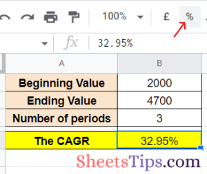
- Step 1- First, create and open a blank spreadsheet and enter Beginning Value in cell B3, Ending Value in B4, Number of periods in cell B5, and lastly The CAGR in cell B7.
- Step 2- Now, let us take the cell C7 for displaying the result, enter the formula =(C4/C3) ^ (1/2)-1and hit Enter.
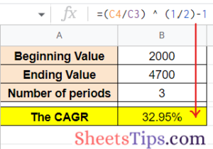
- Step 3- To convert the cell to a percentage, select C7 and press on the Format as percentage button. This will display the compound annual growth rate value in percentage as shown below:
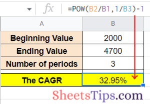
 Another method to calculate the CAGR is to use the Sheets POW function. The syntax for that function is =POW (base, exponent). Now, let us see the steps to using the POW function in order to calculate the compound interest:
- Step 1- Select the cell C8 in your spreadsheet to display the result and enter the formula =POW(C4/C3,1/C5)-1 and hit Enter.
- Step 2- Next, convert the C8 to percentage from Formats as you did for C7.
Google Finance Sheets formulas
The GOOGLE FINANCEfunction is the formula we are talking about here. It accepts a ticker symbol that triggers particular security and returns sophisticated information relating to that security through Google Finance.
It also allows fetching data about both stocks as well as currencies. When applied to research investment opportunities, Google Finance helps in keeping track of stock portfolios, converting and analyzing between currencies, building visualizations and dashboards, performing subsequent calculations, visualizing trends and stock market moves, and much more. The syntax for the GOOGLEFINANCE formula is =GOOGLEFINANCE( ticker, [ attribute ], [ start_date ], [ end_date ], [ interval ]), where,
- ticker is the symbol of the security that represents the data you want to fetch along with the exchange symbol. For example, “NIFTY: GOOG” represents Google stocks from the NIFTY exchange.
- attributeis a single-string parameter that specifies the accessible data with respect to the given ticker. Some of them are “price”, “high”, “low”, “volume”, etc.
- start_date represents the starting date from which you want your data to be fetched or fetch historical data relating to a ticker.
- end_date represents the ending date up to which you want your data to be fetched. You can also alternatively specify the number of days from the start_date for which you want the data to be fetched.
- interval is another optional parameter used to fetch historical data by specifying the intervals between dates of your fetched historical data either “daily” or “weekly”. For data in intervals of 2 days, 3 days, etc., specify a number between 1 and 7.
Google Sheets Investment Calculator
- rate: the fixed amount of interest over a stipulated time. Note here that interest rates are always annual so to calculate the interest rate for quarterly or monthly payments, you will have to divide the rate accordingly, for example, for monthly interest rate, divide by 12, for daily divide by 365, etc.
- number_of_periods: the total number of periodic payments you plan to make.
- payment_amount: the constant amount that you have to pay for each period. This will be the type of payment multiplied by the length of time, for example, for monthly payment over 5 years: 12*5 = 60 periods.
- present_value: This is the current value of the investment. It is an optional parameter and yields zero by default.
- end_or_beginning: This is also optional and is set by 0 by default. 0 indicates that you are paying at the end of each period and 1 indicates that you are paying at the beginning of each payment period.
FAQs on Compound Interest in Google Sheets
Try More: