
Standard Error Google Sheets Guide: Google Sheets is used worldwide to analyze significant volumes of data. These also include mathematical data and understanding the relationship between data from a specific sheet. While analyzing such data and making interpretations, you will need to find patterns and insights that are going to make your data more useful in the future.
Also Read: Java Program to Print Series 6 12 18 24 28 …N
In this guide, you will come across all the important facts about standard deviation and standard errors in Google Sheets. So now without wasting any more time, let’s just quickly jump into these amazing Google Sheets tips.
- What Is the Standard Deviation in Google Sheets and How To Calculate It?
- What Is Standard Error of Mean in Google Sheets?
- How To Find Standard Error in Google Sheets?
- How To Do Standard Error Interpretation in Google Sheets?
- How To Calculate 2SEM in Google Sheets?
- Standard Error Bars in Google Sheets
- How To Create Horizontal Error Bars in Google Sheets?
- FAQs on Standard Deviation in Google Sheets
What Is the Standard Deviation in Google Sheets and How To Calculate It?
To start with, standard deviation is the measure of how clustered or spread out the data is in your data sheet compared to the standard mean. By calculating the standard deviation, you will get a calculative idea of how dispersed your data is. The syntax for the formula to be used is =STDEV(value1, value2, …). This function takes the cell references from your sample and then calculates the standard deviation. You can enter both single cells and ranges of cells as values in it.
Now let’s take the following table as an example, where we have noted the marks of eight students on three different subjects in the following spreadsheet. Let’s see the steps to calculate the standard deviation for each of these subjects and also determine which subject has the most uniform marks.
- Select cell B12, for example where you want to print the result.
- Apply the formula =STDEV(B2:B11) where the function will calculate the standard variation for the numbers in cells B2 to B11 and hit Enter.
- Next, click on the fill handle button and drag it on the cells where you want to calculate the standard deviation, that is the cells C12 and D12 in this example.
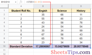
Now you will have the standard deviation for all three subjects. A small number refers to a clustered dataset, whereas a bigger number refers to a dispersed dataset.
What Is the Standard Error of Mean in Google Sheets?
The mean standard error is basically a mathematical method that calculates how far apart the values are in a given data set. The syntax for this mathematical formula is Standard error = s/n, where :
- s is the standard deviation of the sample data.
- n is the size of the sample data.
While translating this equation into Google Sheets, we can use the three formulas: STDEV.S, SQRT, and COUNT. The syntax of all of these formulas is as follows:
- =STDEV.S(dataset), where the dataset is the cell address for the array.
- =SQRT(value), where value is the number for which the square root is calculated. It can also be a cell address.
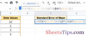
- =COUNT(v1, v2, …), where v1 is the first value or cell range to consider when counted, v2 is the additional ranges ar values can be added depending on circumstances. Now let us put all of these formulas together to find out the standard error on Google Sheets, and have the final syntax as follows: =STDEV.S(range) / SQRT(COUNT(range))
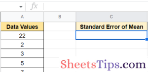
Now, let us see the steps to apply this formula and find out the standard mean error with an example:
- Step 1: First, select the cell where you wish to display the standard error of the mean, and then click on the fx symbol from the toolbar at the top.
- Step 2: Here you will see a menu appear that says “Paste Function”. Click on “Statistical” from the left-hand side of the menu, scroll down on the right-hand side, select “STDEV” and finally “OK”.
- Step 3: Click on the spreadsheet picture, and highlight the numbers you had averaged earlier, just as you did while taking the average, and press enter followed by “OK” to calculate the standard deviation of the selected values.
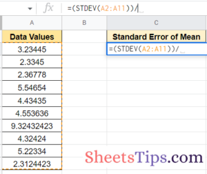
- Step 4: Keeping the cursor still on the same cell, click in the formula bar at the top of the spreadsheet (the white box next to the “=” sign) to put the cursor in that bar so you can edit the formula.
- Step 5: Put a “(” before STDEV and a “)” at the end. Next, put a “/” sign to indicate you are dividing this standard deviation and place two sets of parentheses “(())” after the division symbol. Next, place the cursor in the middle of these parentheses.
- Step 6: Now click on the fx symbol, select “Statistical” on the left-hand menu, and “Count” on the right-hand menu.
- Step 7: Again, click on the spreadsheet picture in the pop-up box, highlight the list of numbers averaged, hit enter, and “OK” as you did before.
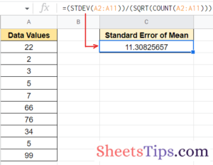
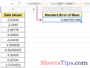
- Step 8: Now, move the cursor between the two sets of parentheses, type “SQRT” and press enter. In the fx bar, enter =(STDEV (A1:A2))/(SQRT (COUNT (A1:A2)) to calculate the standard error of the mean for the values in cells A1 to A2.
How To Do Standard Error Interpretation in Google Sheets?
To interpret the standard error in Google Sheets, there are essentially two important things you need to follow to correctly interpret the value of the standard mean error. These are:
1) Larger the SEM Value more spread out the values are:
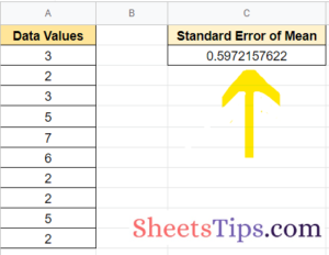
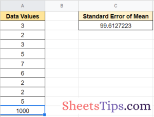
If we see that the difference between the values in a table tends to be larger, then the SEM value will increase. In the first sample dataset, the values are quite close to each other, so we see that the SEM value is smaller. In the second dataset, we changed the value significantly larger than the others, which made the SEM value rise from 0.8386714776 to 49.37885218.
2) SEM Value Increases with smaller sample sizes:
As the number of values increases, the SEM value will proportionally decrease. In the first sample dataset, there are 20 values in the dataset, while in the second one, there are only 9. This will make the SEM value change from 0.8386714776 to 1.490329255. If the extra figures were outliers instead, the SEM number would have increased.
How To Calculate 2SEM in Google Sheets?
To understand this concept better, we have a set of data with random values as an example. Here are the steps that will help you find the standard error of the mean in Google Sheets:
- Step 1: First, we’ll have to divide the formula into two main parts. The first part will have the STDEV.S formula, while the second one will have the SQRT and the COUNT formula. To start with, select the cell where you want to input the formula and display the error.
- Step 2: First, input the =STDEV.S ( part of the formula, select the cell address range A2: A21 and finish this off by adding a closing bracket and a division slash (/).
- Step 3: Now, we will nest the COUNT formula inside the SQRT formula. So type the first part as =SQRT( of the formula, followed by the COUNT( keyword, and then input the same range in the formula as you did in the STDEV.S formula, finishing it with a closing bracket. Just check and make sure the number of closing brackets is the same as the number of opening brackets.
- Step 4: Finally, press Enter to execute the formula.
Standard Error Bars in Google Sheets
Standard Error bars are used in charts to visually show the error that can be expected with a given value. There are three main types of error bars in Google Sheets, namely, percent, constant and standard deviation. Here are the steps that you need to follow to insert a column chart to determine the standard error in Google Sheets:
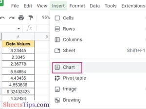
- Step 1: Select the dataset including the headers, click on the Insert tab and click on the Chart option, or you can also click on the chart icon in the toolbar.
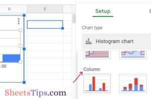
- Step 2: By default, it will insert a Pie Chart, double click on it to open the Chart editor pane on the right-hand side, click on the Chart Type drop-down and select the Column Chart option.
 The above steps will insert a column chart that will look something like the one shown below.
 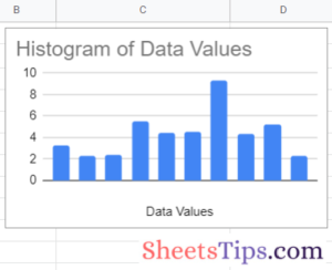 Now, let us see the steps to adding the error bars to this column chart:
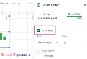
- Step 1: Double-click on the chart to open the Chart Editor pane on the right-hand side and click on “Customize”. Under the Customize menu, click on the arrow beside the Series option.

- Step 2:Scroll down further and click on the “Error bars’ option. In the Type drop-down, select Percentage and enter 10 in the Value field.
 By following the above steps, you will see the error bars on all the columns of the chart where the evaluations are located at the top of the column bars.
  In the above example, we specified the error bar to cover +/-10% of each value in the column, which is also known as the percentage type of error bar.
How To Create Horizontal Error Bars in Google Sheets?
You know, you can always experiment with charts according to your preferences. Similarly, you can also insert horizontal charts into your data set. For this, simply first demarcate two columns that will represent your mean average and standard mean as per the steps already mentioned before.
Next, select the columns you want to display in the chart and follow the steps to insert the chart as mentioned above. Just select horizontal bars instead of columns and do the rest of the cell-specific configurations accordingly.

FAQs on Standard Error in Google Sheets
Try More: