
Spreadsheets provide great analysis skills, but they occasionally lack that extra layer of understanding. It’s difficult to summarise or draw conclusions from a basic tabular spreadsheet view when there’s a large amount of data.
Also Read: Cloud Computing Notes
The pivot table comes into play. Most Excel expert users rely on pivot tables as their bread and butter, but Google Sheets has a similar capability, so you can utilize pivot tables while staying in G Suite. In this tutorial, we’ll go through how to create pivot tables using Google Sheets Tips and Tricks.
- What Are Pivot Tables?
- How to Make a Google Sheets Pivot Table?
- How to Refresh a Google Sheets Pivot Table?
What Are Pivot Tables?
A spreadsheet, in its most basic form, is just a collection of columns and rows. Cells are generated when a column and a row intersect. You may apply formulas to log data within these cells, and when your spreadsheet is tiny, the numbers are easy to see and comprehend.
However, when your spreadsheet grows in size, making conclusions demands a little more muscle. This is where pivot tables come into play. A pivot table summarises a huge amount of data.
So, you can take a two-dimensional table and pivot it around a data aggregate to add a third dimension. That’s how you make a pivot table. This allows you to see the big picture, draw meaning from enormous amounts of data, and uncover new insights.
While many of these insights may be obtained using mathematics, the pivot table allows you to condense them in a fraction of the time—and with less danger of human error. Furthermore, if your employer requests a new report based on the same data set, you may produce it with a few clicks rather than beginning from scratch.
How to Make a Google Sheets Pivot Table?
The methods below demonstrate how to quickly and easily construct a pivot table in Google Sheets using a small dataset.
Step 1: Access your data set
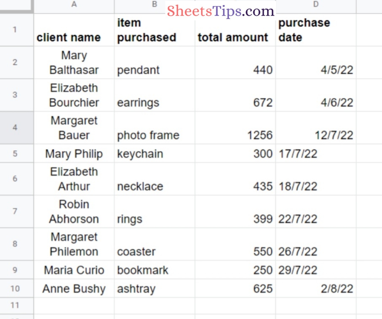
Open the Excel file containing your raw data and click anywhere inside the table.
Assume your data comprises distinct sales entries for your small business, along with customer name and date in this example.
Step 2: Navigate to the Menu and select an insert.
Navigate to the Google Sheets Menu, select Insert, and click Pivot Table.
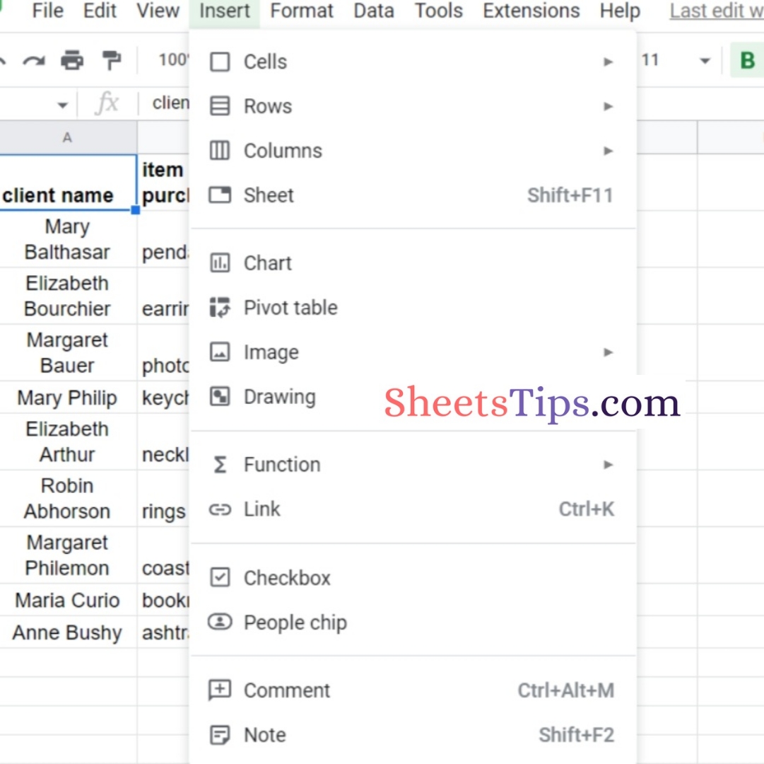
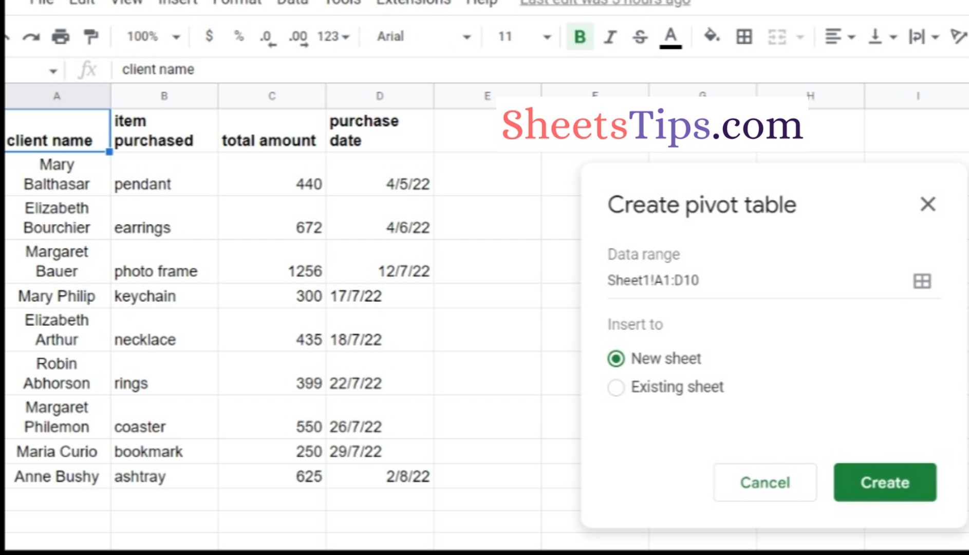
Then, choose whether to insert the pivot table into the existing sheet or a new sheet.
When you create a new sheet, the newly generated tab is called Pivot Table 1. (or Pivot Table 2, Pivot Table 3, and so on as you add more).
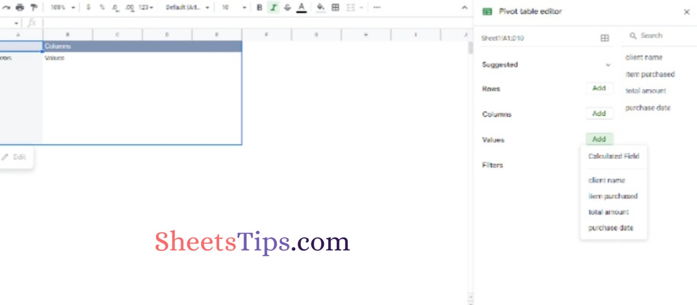
Step 3: Insert the desired row and value data.
Next, go to Values and click Add.
And voila! You just created your first pivot table in a few quick and easy steps.
Now, let’s look at some of the essential components and operations of pivot tables to help you understand them better.
Rows
Within the Pivot table editor, click Add under the Rows category to get a list of your table’s column headings.
Choose anyone, and the pivot table will incorporate the unique data from your chosen column as row headers in your pivot table.
The rows of the category fields display as a distinct list on the pivot table’s left side.
Columns
When you add columns, the values data will be presented as aggregated information for each column.
The fields in the Columns section displayed as a distinct list in the pivot table’s top box.
Values
Click on Values to view the same list of column headings, and picking one will cause the pivot table to summarise that particular column.
Fields in the Values category appear as numbers in the pivot table’s main box.
For example, you could want to total or average your income, or you might want to count the text values in a column.
You obtain summary data when you add values, such as an aggregated view of all the combined individual values from each row into a single number.
You can also easily drag and drop the fields and move them around within the Pivot table editor, for example, swapping the fields in the Rows section for the fields in the Columns section. As you move your fields, the pivot table will automatically modify your data display.
Totals
You may enable or disable the totals in any of your pivot tables’ values columns.
Toggle the box next to the Show totals option in the Rows and Columns category of the Pivot table editor.
How to Refresh a Google Sheets Pivot Table?
In general, you don’t need to refresh pivot tables in Google Sheets because they update immediately when you modify the information on the sheets with your original data sets.
However, there may be times when you need to manually refresh your pivot tables if the data does not update automatically.
The following are a few reasons why your pivot tables do not update automatically, as well as solutions to the problems.
Reason 1: You Have Filters in Your Pivot Tables
If your pivot table in Google Sheets incorporates filters, your data will not be updated when you modify the original data values.
To remove the filters from your pivot table, click the cross sign below all of the fields beneath the Filters option in the Pivot table editor.
Changes to the original data set should be reflected in your pivot table. Then, within the Pivot table editor, re-add the filters by selecting the Add button in the Filters category.
Reason 2: You’re Inserting New Rows Outside the Range of the Pivot Table
Pivot tables employ data from specified cell ranges in the worksheet of your source dataset. If you insert new rows and data beyond the pivot table’s range, the information will have no effect on the pivot table.
Ensure that your newly added rows are inside the pivot table’s range by providing extra blank rows for data that you may need to add later or by adjusting the range in the pivot table editor.
Leaving blank rows in your original worksheet, on the other hand, may result in blank rows on your pivot tables, which may not be aesthetically appealing.
You may set a filter to show just rows with values, or you can modify the range directly to include your new rows, and your pivot table will immediately refresh with the new rows.
Reason 3: Today, Random, and Other Functions Are Included in Your Original Dataset
Any modifications to your original dataset will not update your pivot tables if the original worksheet contains refreshable functions like TODAY, RANDOM, and others.
Avoid including these functions in your original dataset if possible, or utilize cloud pivot tables to automatically update your pivot tables independent of the functions present in the source data sheet.
Essentially, updating your pivot table entails modifying the Pivot table editor or adding or removing particular information from your source datasheets.
As long as your original dataset sheet does not contain any of the flaws listed below, both approaches will automatically update your pivot tables to the required version.
Tip: Take before and after screenshots of your pivot tables to evaluate whether modifications to the data source had any influence on your pivot table.
Conclusion
Google Sheets’ pivot tables enable you to quickly summarize, analyze, and extract insights from your data.
With pivot tables, you receive a powerful tool that can help you uncover the potential of your data. This allows you to extract information that your company’s stakeholders can readily exploit without the need for sophisticated algorithms, saving you a significant amount of time and work.
Learn how to utilize pivot tables to make the process of data gathering, analysis, organization, summarization, and report generation easier, faster, and more reliable.
Pivot tables are simple to play with. After you’ve mastered the fundamentals, try taking things to the next level by adding additional fields in different portions of the Pivot table editor to see what type of data you’ll obtain.
Refer: AUBANK Pivot Calculator