
Simple Instructions for Using a Google Sheets Expense Template: The best way to achieve your financial goals is to maintain a budget, keep track of it, and plan your finances accordingly. Good news! You do not require any additional fancy apps for it because Google Sheets provides you with its built-in tracker and budget management applications to help you with the same.
You can either create your own expense tracker from scratch and customize it as per your requirements, or download it from the ready-made templates. So, let’s quickly see how to track expenses in Google Sheets using these Google Sheet tips.
- What Is a Google Sheets Expense Report Template?
- How To Make an Expense Tracker in Google Sheets?
- Google Sheets Income and Expense Tracker
- How To Make a Spending Tracker in Google Sheets from Scratch?
- Monthly Expense Tracker Google Sheets Template
What Is a Google Sheets Expense Report Template?
The Google Sheets Expense Tracker templates are basically ready-made tools that help us keep track of our income and expenditures and create reports for the same. We can keep a record of our earnings and spending on a monthly or annual basis.
Google Sheets provides us with both paid and free versions for expense tracking. Each template functions differently, so you get a huge variety of options to choose from, considering which template suits your needs the best. They also provide additional charts to help you visualize your totals at the end of each month.
How To Make an Expense Tracker in Google Sheets?
As already mentioned before, Google Sheets provides you with two main options to keep track of your income and expenditure absolutely without cost or third-party apps. These are:
- Google Sheets has in-built monthly expenses and budget templates.
- Creating our very own Google Sheets expense tracker with customized options
You get to choose templates from 1 month to a year and do your expense mapping plus budgeting over there. You can choose from a single sheet to a one-tab per month template. You can also opt for the new version that provides category selection.
Google Sheets Income and Expense Tracker
After reading the previous stuff, the first thing that comes to your mind is, Does Google Sheets have a budget template? Well, Google Sheets has an array of templates to choose from depending upon your payment styles and needs. Let’s see the steps now:
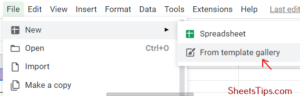
- Step 1: Open Google Sheets and navigate to the file menu. Next, click on the New tab and select From template gallery.
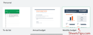
- Step 2: This will open the Google Sheets Template Gallery. Next, under the Personal section, click on the Monthly Budget thumbnail.
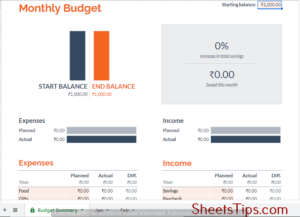
- Step 3: This will open the template for tracking monthly budgets. Here’s how it looks:
- Step 4: Once the monthly budget template is open in front of you, you will see that there are two major tabs in the workbook, namely:
- Summary
- Transactions
In the transactions tab, you get to enter your daily income and expenditure data. You insert the income details on the left and expenses on the right. You get four columns for each section. These are:
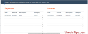
- Date: You enter the date of transactions here.
- Amount: This field holds the amount received or paid.
- Description: This field explains the purpose of the transaction.
- Category: This describes the payment category.
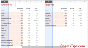
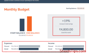
- Step 5: Make sure you choose the most appropriate category from the drop-down list because this is going to be used later on while summarising your income and expenditures and will be displayed in the Summary tab. The Summary tab is basically like a brief dashboard that displays a gist of your income and expenses along with a basic view of your cash flow.
The Summary tab basically holds the following data:
- A place to enter the starting balance or salary for the month.
- A bar displaying the starting balance versus the month-end balance
- A specific place that shows the approximate percentage of your savings in the current month.
- Two bar charts to show your planned vs. actual savings or expenses.
- A category-wise summary chart for your income in the current month.
- Category-wise summary of your total expenditure for the current month.
Monthly Expense Tracker Google Sheets Template
Once you have successfully set up the monthly budget tracker template, let’s see the steps on how to use it properly to track your income and expenses:
- Step 1: First, clear out all the transactions from the Transactions tab. Select all the rows from both tables and press the Delete key on your keyboard.
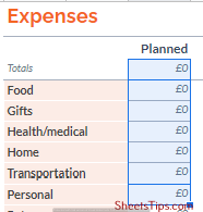
- Step 2: Now, go to the Summary tab and change the categories in columns B and H to suit your needs.
- Step 3: Next, delete the planned values given in cells and place a 0 instead.
- Step 4: Now your monthly money tracking template is all ready to be duplicated. Every month, just make a copy of this file by going to the File menu followed by Make a copy.
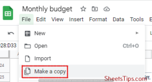
- Step 5: In case you are wondering about How to make an expense report on Google Sheets? just rename the file as per the month’s name to make it easier for you to track records in the future.
- Step 6: Next, start by entering your starting balance of the month first and filling in your budget in each category, but make sure to keep the limit lower than the starting balance. Also, fill in your planned expenses in the planned columns of both tables.
- Step 7: Navigate to the Transactions tab next and start entering your income and expenses.
- Step 8: When you’re finished, click on the Summary tab to see your income and expenses categorised and displayed in their respective actual sums.
How To Make a Spending Tracker in Google Sheets From Scratch?
If you prefer creating your very own expense tracker and customizing it in your way, then you are absolutely free to do so. So, let us now see how to create a Google Sheets transaction tracker from scratch:
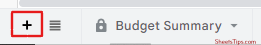
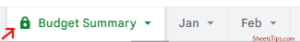
- Step 1: First, we need to rename the Transactions and Summary tabs that we are going to work with. Next, create a second worksheet by clicking on the ‘+’ icon next to Sheet1.
Initially, you can rename Sheet1 to Budget Summary and Sheet2 to the month’s name, and later on, just duplicate this tab and rename it to the new current month’s name, for every month.
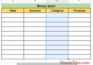
- Step 2: Creating the Outline for Transactions Sheet – Let’s start by creating a basic skeleton of our template for the ‘Transactions’ tab and enter all our plus and minus transactions.
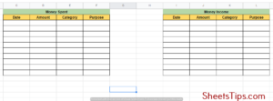
Format column D cells to the ‘Currency’ format by first selecting the cells and going to the Format option, followed by Number and Currency.
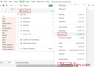
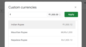
Also, make sure you change the currency to your country’s one by clicking on Custom currency and selecting your country’s name from the drop-down list of regions.
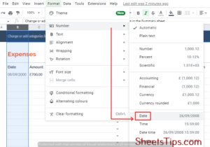
Next, Format column A cells to the ‘Date’ format in the same process as mentioned above. We can keep the Category column to be updated once the Budget Summary Sheet is ready.
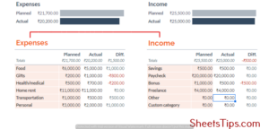
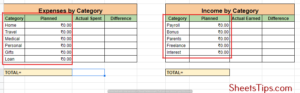
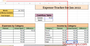
- Step 3: Creating the Outline for the Budget Summary Sheet- You can take reference from the image given below to draw a basic outline of the expense income category tables, cash flow tables, etc., and add the categories as per your needs.
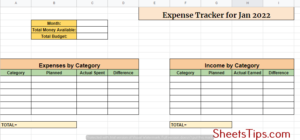
Format the cells B11: D18, G11: I18, C4: C5, and F6:F7 to the Currency format and add 0s to the Planned columns in both the income and expense category tables.
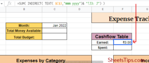
- Step 4: Adding Formulas in the Cash Flow Table- Let’s start by entering the formulas for the Cash Flow table in cells F6 and F7:
- F6: =SUM( INDIRECT( TEXT( $C$3,”mmm yyyy”) &” !J3: J”) ), holding the value for total money income throughout the month and we will have to pull this value from the column J of our Transactions tab.
- F7: =SUM( INDIRECT( TEXT( $C$3,”mmm yyyy”) &”!D3: D”) )
Next, we need to sum up all the values in J3: J to get the total amount earned. Use the formula: =SUM(‘Jan 2021’!J3:J)
Next, set an indirect function for J3: J to make it dynamic so that we can add more tabs for different months in the future. Use the formula: =SUM( INDIRECT( TEXT( $C$3,”mmm yyyy”)& “!J3: J”) )
Step 5: Adding Formulas to the Expense and Income Category Tables-The Category tables contain expense entries, planned expenses, and the difference between the two.
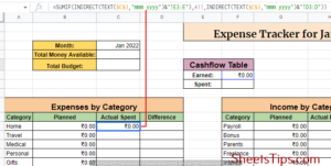
- The Spent column displays the total expenditure towards each category. Let us start with the first category (the Shopping category). In C11, enter the formula: =SUMIF(INDIRECT(TEXT($C$3,”mmm yyyy”)&”!E3:E”),A11,INDIRECT(TEXT($C$3,”mmm yyyy”)&”!D3:D”)). The output in cell C11 will be something like this:
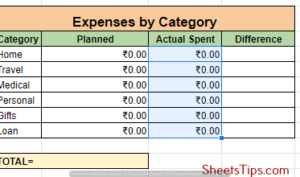
Copy the formula to cell C17 by using the fill handle) and this is how the C11:C17 will look:
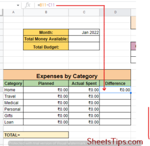
- The Difference column cells D11:D17 display the difference between the Planned and Actual expenses with respect to each category. So in cell D11 enter the formula: =B11-C11 and copy it down to D17.
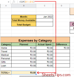
- The total row will calculate the totals in row 18, so assign B18 the formula: =SUM(B11:B16) and copy it up to cell D18 by using the fill handle.
This is how your Expenses by Category table looks at this point:
Repeat the same for the Income by Category table using the formulas:
- H11: =SUMIF(INDIRECT(TEXT($C$3,”mmm yyyy”)&”!K3:K”),F11,INDIRECT(TEXT($C$3,”mmm yyyy”)&”!J3:J”)) and copy to cell H17
- I11:= H11-G11 and copy this to cell I17
- G18:=SUM(G11:G17) and copy this to cell I18.
This is what your final Income by Category table looks like at this point:
Step 6: Adding Formulas to the Summary Table-
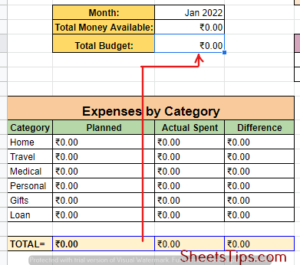
- In cell C4, enter the formula for H18 to give you the total amount earned for the given month. i.e =H18
- In cell C5, put =B18 to get the total budget for the month.
Ensure the total budget does not exceed the total income amount –
- Click on cell C5 and got to Data followed by Data Validation.
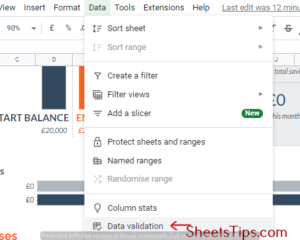
- In the Data Validation dialog box, go to Criteria and select Number from the dropdown list.
- Next, click on less than or equal to and enter =C4 in the next input box.
- Finally, click Save.
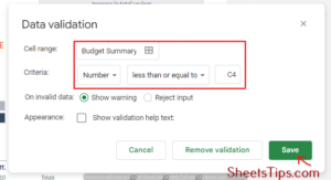
2. To ensure we don’t accidentally enter a Transaction sheet category that is not reflected in the Summary sheet.
- Select all the cells from column E starting from cell Es3 first.
- Next, go to Data, followed by Data Validation, select Criteria, and click on List from Range from the dropdown list that appears.
- Enter the range of category list in the next input box that is Budget Summary’!$A$11:$A$17’.

- Next, put a check on the box beside the Show validation help text, and in the input box below type”Please select a category from the available list”.

- Lastly, click Save.
Step 8: Protecting Cells- Lastly, we must make sure that certain cells in the expense tracker are protected to avoid accidental changes. Follow the steps given below:
- Right-click on this sheet’s tab and select ‘Protect Sheet’.
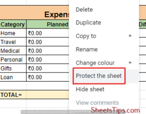
- You will see the Protected sheets and ranges window on the right check the box for ‘Except certain cells’.
- In the input box present under this checkbox, type the cell-range you don’t aim to protect i.e., B11:B17.

- Click on Add another range and in the new input box, enter range G11:G17.
- Next, click on Add another range and enter the range C3 in the new input box.

- Finally, click Ok followed by the Set Permissions button, and Show a warning when editing this range pop up.

- Lastly, click Done to finish.
Now, your whole sheet is protected except for B11:B17, G11:G17, and C3, where the user will input.